
Chapter 3
Hard-Surface Modeling
Creating 3D models in computer graphics is an art form and a discipline unto itself. It takes years to master and requires an understanding of form, composition, anatomy, mechanics, and gestures. It’s an addictive art that never stops evolving. With a firm understanding of how the tools work, you can master the art of creating 3D models.
The Autodesk® Maya® software supports three types of surfaces: polygon, NURBS, and subdivisions. Each is quite different and has its strengths and weaknesses. There are few restrictions when working with polygons, and for this reason they are more popular than NURBS and subdivisions as a modeling tool. Ultimately, NURBS and subdivision surfaces can be converted to polygons, allowing you to take advantage of the strengths of both. This chapter walks you through the different components of each surface type. Once you have a solid understanding of the surfaces, we’ll demonstrate various techniques for building hard-surface models. We’ll use all three surface types to create a bicycle.
In this chapter, you will learn to
- Understand polygon geometry
- Understand NURBS surfaces
- Understand subdivision surfaces
- Employ image planes
- Model with NURBS surfaces
- Model with polygons
Understanding Polygon Geometry
Polygon geometry refers to a surface made up of polygon faces that share edges and vertices. A polygon face is a geometric shape consisting of three or more edges. Vertices are points along the edges of polygon faces, usually at the intersection of two or more edges.
Many tools are available that allow you to make arbitrary changes (such as splitting, removing, and extruding) to polygon faces. Polygons are versatile. They can be used to create hard-surface models, such as vehicles, armor, and other mechanical objects, as well as organic surfaces, such as characters, creatures, and other natural objects. Before you get started working on the bicycle, it’s a good idea to gain an understanding of the basic components of a polygon surface.
Polygon Vertices
A polygon is a surface constructed using three or more points known as vertices. The surface between these vertices is a face. A mesh is a series of faces that share two or more vertices. The most common way to create a polygon surface is to start with a primitive (such as a plane, sphere, or cube) and then use the numerous editing tools to shape the primitive gradually into the object that you want to create.
When all of the vertices of a polygon are along a single plane, the surface is referred to as planar. When the vertices are moved to create a fold in the surface, the surface is referred to as nonplanar (see Figure 3.1). It’s usually best to keep your polygon surfaces as planar as possible. This strategy helps you to avoid possible rendering problems, especially if the model is to be used in a video game. As you’ll see in this chapter, you can use a number of tools to cut and slice the polygon to reduce nonplanar surfaces.

Figure 3.1 Moving one of the vertices upward creates a fold in the surface.
Polygon Edges
The line between two polygon vertices is an edge. You can select one or more edges and use the Move, Rotate, and Scale tools to edit a polygon surface. Edges can also be flipped, deleted, or extruded. Having this much flexibility can lead to problematic geometry. For instance, you can extrude a single edge so that three polygons share the same edge (see Figure 3.2).

Figure 3.2 Three polygons are extruded from the same edge.
This configuration is known as a nonmanifold surface, and it’s a situation to avoid. Some polygon-editing tools in Maya do not work well with nonmanifold surfaces, and they can lead to rendering and animation problems. Another example of a nonmanifold surface is a situation where two polygons share a single vertex but not a complete edge, creating a bow-tie shape (see Figure 3.3).

Figure 3.3 Another type of nonmanifold surface is created when two polygons share a single vertex.
Polygon Faces
The actual surface of a polygon is known as a face. Faces are what appear in the final render of a model or animation. There are numerous tools for editing and shaping faces, which are explored throughout this chapter and the next one.
Take a look at Figure 3.4. You’ll see a green line poking out of the center of each polygon face. This line indicates the direction of the face normal; essentially, it’s where the face is pointing.

Figure 3.4 The face normals are indicated by green lines pointing from the center of the polygon face.
The direction of the face normal affects how the surface is rendered; how effects such as dynamics, hair, and fur are calculated; and other polygon functions. Many times, if you are experiencing strange behavior when working with a polygon model, it’s because there is a problem with the normals (see Figure 3.5). You can usually fix this issue by softening or reversing the normals.

Figure 3.5 The normal of the second polygon is flipped to the other side.
Two adjacent polygons with their normals pointing in opposite directions is a third type of nonmanifold surface. Try to avoid this configuration.
Working with Smooth Polygons
![]()
There are two ways to smooth a polygon surface: you can use the Smooth operation (from the Modeling menu set, choose Mesh ➣ Smooth), or you can use the Smooth Mesh Preview command (select a polygon object, and press the 3 key).
When you select a polygon object and use the Smooth operation in the Mesh menu, the geometry is subdivided. Each level of subdivision quadruples the number of polygon faces in the geometry and rounds the edges of the geometry. This also increases the number of polygon vertices available for manipulation when shaping the geometry (see Figure 3.6).

Figure 3.6 From left to right, a polygon cube is smoothed two times. Each smoothing operation quadruples the number of faces, increasing the number of vertices available for modeling.
When you use the smooth mesh preview, the polygon object is actually converted to a subdivision surface, or subD. Maya uses the OpenSubdiv Catmull-Clark method for subdividing the surface. You can read more about subdivision surfaces later in this chapter in the section “Using Subdivision Surfaces.”
When a polygon surface is in smooth mesh preview mode, the number of vertices available for manipulation remains the same as in the original unsmoothed geometry; this simplifies the modeling process.
- To create a smooth mesh preview, select the polygon geometry and press the
3key. - To return to the original polygon mesh, press the
1key. - To see a wireframe of the original mesh overlaid on the smooth mesh preview (see Figure 3.7), press the
2key.

Figure 3.7 This image shows the original cube, the smooth mesh preview with wireframe, and the smooth mesh preview without wireframe.
The terms smooth mesh preview and smooth mesh polygons are interchangeable; both are used in this book and in the Maya interface.
When you render polygon geometry as a smooth mesh preview using mental ray®, the geometry appears smoothed in the render without the need to convert the smooth mesh to standard polygons or change it in any way. This makes modeling and rendering smooth and organic geometry with polygons much easier.
Understanding NURBS
NURBS is an acronym that stands for Non-Uniform Rational B-Spline. As a modeler, you need to understand a few concepts when working with NURBS, but the software takes care of most of the advanced mathematics so that you can concentrate on the process of modeling.
Early in the history of 3D computer graphics, NURBS were used to create organic surfaces and even characters. However, as computers have become more powerful and the software has developed more advanced tools, most character modeling is accomplished using polygons and subdivision surfaces. NURBS are more ideally suited to hard-surface modeling; objects such as vehicles, equipment, and commercial product designs benefit from the types of smooth surfacing produced by NURBS models.
All NURBS objects are automatically converted to triangles at render time by the software. You can determine how the surfaces will be tessellated (converted into triangles) before rendering, and you can change these settings at any time to optimize rendering. This gives NURBS the advantage that their resolution can be changed when rendering. Models that appear close to the camera can have higher tessellation settings than those farther away from the camera.
One of the downsides of NURBS is that the surfaces themselves are made of four-sided patches. You cannot create a three- or five-sided NURBS patch, which can sometimes limit the kinds of shapes that you can make with NURBS. If you create a NURBS sphere and use the Move tool to pull apart the control vertices at the top of the sphere, you’ll see that even the patches of the sphere that appear as triangles are actually four-sided panels (see Figure 3.8).
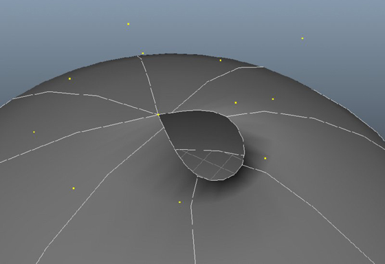
Figure 3.8 Pulling apart the control vertices at the top of a NURBS sphere reveals that one side of each patch had been collapsed.
Understanding Curves
All NURBS surfaces are created based on a network of NURBS curves. Even the basic primitives, such as the sphere, are made up of circular curves with a surface stretched across them. The curves themselves can be created several ways. A curve is a line defined by points. The points along the curve are referred to as curve points. Movement along the curve in either direction is defined by its U-coordinates. When you right-click a curve, you can choose to select a curve point. The curve point can be moved along the U-direction of the curve, and the position of the point is defined by its U-parameter.
Curves also have edit points that define the number of spans along a curve. A span is the section of the curve between two edit points. Changing the position of the edit points changes the shape of the curve; however, this can lead to unpredictable results. It is a much better idea to use a curve’s control vertices to edit the curve’s shape.
Control vertices (CVs) are handles used to edit the curve’s shapes. Most of the time, you’ll want to use the control vertices to manipulate the curve. When you create a curve and display its CVs, you’ll see them represented as small dots. A small box indicates the first CV on a curve; the letter U indicates the second CV.
Hulls are straight lines that connect the CVs; they act as a visual guide. Figure 3.9 displays the various components.

Figure 3.9 The top image shows a selected curve point on a curve, the middle image shows the curve with edit points displayed, and the bottom image shows the curve with CVs and hulls displayed.
The number of CVs per span minus one determines the degree of a curve. In other words, a three-degree (or cubic) curve has four CVs per span. A one-degree (or linear) curve has two CVs per span (see Figure 3.10). Linear curves have sharp corners where the curve changes directions; curves with two or more degrees are smooth and rounded where the curve changes direction. Most of the time, you’ll use either linear (one-degree) or cubic (three-degree) curves.

Figure 3.10 A linear curve has sharp corners.
You can add or remove a curve’s CVs and edit points, and you can also use curve points to define a location where a curve is split into two curves or joined to another curve.
The parameterization of a curve refers to the way in which the points along the curve are numbered. There are two types of parameterization:
Uniform Parameterization A curve with uniform parameterization has its points evenly spaced along the curve. The parameter of the last edit point along the curve is equal to the number of spans in the curve. You also have the option of specifying the parameterization range between 0 and 1. This method is available to make Maya more compatible with other NURBS modeling programs.
Chord Length Parameterization Chord length parameterization is a proportional numbering system that causes the length between edit points to be irregular. The type of parameterization you use depends on what you are trying to model. Curves can be rebuilt at any time to change their parameterization; however, this will sometimes change the shape of the curve.
You can rebuild a curve to change its parameterization (using the Modeling menu set under Curves ➣ Rebuild). It’s often a good idea to do this after splitting a curve or joining two curves together, or when matching the parameterization of one curve to another. By rebuilding the curve, you ensure that the resulting parameterization (Min and Max Value attributes in the curve’s Attribute Editor) is based on whole-number values, which leads to more predictable results when the curve is used as a basis for a surface. When rebuilding a curve, you have the option of changing the degree of the curve so that a linear curve can be converted to a cubic curve and vice versa.
Understanding NURBS Surfaces
NURBS surfaces follow many of the same rules as NURBS curves since a network of curves defines them. A primitive, such as a sphere or a cylinder, is simply a NURBS surface lofted across circular curves. You can edit a NURBS surface by moving the position of the surface’s CVs (see Figure 3.11). You can also select the hulls of a surface, which are groups of CVs that follow one of the curves that define a surface (see Figure 3.12).

Figure 3.11 The shape of a NURBS surface can be changed by selecting its CVs and moving them with the Move tool.

Figure 3.12 Hulls can be selected and repositioned using the Move tool.
NURBS curves use the U-coordinates to specify the location of a point along the length of the curve. NURBS surfaces add the V-coordinate to specify the location of a point on the surface. Thus a given point on a NURBS surface has a U-coordinate and a V-coordinate. The U-coordinates of a surface are always perpendicular to the V-coordinates of a surface. The UV coordinate grid on a NURBS surface is just like the lines of longitude and latitude drawn on a globe.
Just like NURBS curves, surfaces have a degree setting. Linear surfaces have sharp corners (see Figure 3.13), and cubic surfaces (or any surface with a degree higher than 1) are rounded and smooth. Often a modeler will begin a model as a linear NURBS surface and then rebuild it as a cubic surface later (Surfaces ➣ Rebuild ➣ ❒).

Figure 3.13 A linear NURBS surface has sharp corners.
You can start a NURBS model using a primitive, such as a sphere, cone, torus, or cylinder, or you can build a network of curves and loft surfaces between the curves or any combination of the two. When you select a NURBS surface, the wireframe display shows the curves that define the surface. These curves are referred to as isoparms, which is short for “isoparametric curve.”
A single NURBS model may be made up of numerous NURBS patches that have been stitched together. This technique was used for years to create CG characters, but now most artists favor polygons or subdivision surfaces. When you stitch two patches together, the tangency must be consistent between the two surfaces to avoid visible seams. It’s a process that often takes some practice to master (see Figure 3.14).

Figure 3.14 A character is created from a series of NURBS patches stitched together.
Surface Seams
Many NURBS primitives have a seam where the end of the surface meets the beginning. Imagine a piece of paper rolled into a cylinder. At the point where one end of the paper meets the other end, there is a seam. The same is true for many NURBS surfaces that define a shape. When you select a NURBS surface, the wireframe display on the surface shows the seam as a bold line. You can also find the seam by selecting the surface and choosing Display ➣ NURBS ➣ Surface Origins (see Figure 3.15).

Figure 3.15 The point on a NURBS surface where the seams meet is indicated by displaying the surface origins.
The seam can occasionally cause problems when you’re working on a model. In many cases, you can change the position of the seam by selecting one of the isoparms on the surface (right-click the surface and choose Isoparm) and choosing Surfaces ➣ Move Seam.
NURBS Display Controls
You can change the quality of the surface display in the viewport by selecting the surface and pressing 1, 2,or 3 on the keyboard:
- Pressing the
1key displays the surface at the lowest quality, which makes the angles of the surface appear as corners. - Pressing the
2key gives a medium-quality display. - Pressing the
3key displays the surface as smooth curves.
None of these display modes affects how the surface will look when rendered, but choosing a lower display quality can help improve performance in heavy scenes. The same display settings apply for NURBS curves as well. If you create a cubic curve that has sharp corners, remember to press the 3 key to make the curve appear smooth.
Using Subdivision Surfaces
![]()
The Maya subdivision surfaces are very similar to the polygon smooth mesh preview. The primary distinction between smooth mesh preview and subdivision surfaces (subDs) is that subdivision surfaces allow you to subdivide a mesh to add detail only where you need it. For instance, if you want to sculpt a fingernail at the end of a finger, using subDs you can select just the tip of the finger and increase the subdivisions. Then you have more vertices to work with just at the fingertip, and you can sculpt the fingernail.
Most subD models start out as polygons and are converted to subDs only toward the end of the modeling process. You should create UV texture coordinates while the model is still made of polygons. They are carried over to the subDs when the model is converted.
So why are subDs and smooth mesh preview polygons so similar, and which should you use? SubDs have been part of Maya for many versions. Smooth mesh preview polygons have only recently been added to Maya, and thus the polygon tools have evolved to become very similar to subDs. You can use either type of geometry for many of the same tasks; it’s up to you to decide when to use one rather than another.
When you convert a polygon mesh to a subdivision surface, you should keep in mind the following:
- Keep the polygon mesh as simple as possible; converting a dense polygon mesh to a subD significantly slows down performance.
- You can convert three-sided or n-sided (four-or-more-sided) polygons into subDs, but you will get better results and fewer bumps in the subD model if you stick to four-sided polygons as much as possible.
- Nonmanifold geometry is not supported. You must alter this type of geometry before you are allowed to do conversion.
Employing Image Planes
![]()
Image planes refer to implicit surfaces that display an image or play a movie. They can be attached to a Maya camera or free floating. The images themselves can be used as a guide for modeling or as a rendered backdrop. You can alter the size of the planes, distorting the image, or use Maintain Pic Aspect Ratio to prevent distortion while scaling. Image planes can be rendered using Maya software or mental ray. In this section, you’ll learn how to create image planes for Maya cameras and how to import custom images to use as guides for modeling a bicycle.
It’s not unusual in the fast-paced world of production to be faced with building a model based on a single view of the subject. You’re also just as likely to be instructed to blend together several different designs. You can safely assume that the director has approved the concept drawing that you have been given. It’s your responsibility to follow the spirit of that design as closely as possible with an understanding that the technical aspects of animating and rendering the model may force you to make some adjustments. Some design aspects that work well in a two-dimensional drawing don’t always work as well when translated into a three-dimensional model. Building a hard-surface model from real-world photos, as we’ll do with the bicycle, can be easier if you know that all of the pieces and parts have been designed to fit together.
Image planes are often used as a modeling guide. They can be attached to a camera or be free floating and have a number of settings that you can adjust to fit your own preferred style. The following exercise walks you through the steps of adding multiple image planes:
- Create a new scene in Maya.
- Switch to the front view. From the Create menu, choose Free Image Plane (see Figure 3.16).
- A dialog box will open; browse the file directory on your computer, and choose the
bicycleFront.jpgimage from thechapter3sourceimagesdirectory at the book’s web page atwww.sybex.com/go/masteringmaya2016. - The front-view image opens and appears in the viewport. Select the image plane, and open the Attribute Editor (see Figure 3.17).
-
In the Image Plane Attributes section, you’ll find controls that change the appearance of the plane in the camera view. Make sure that the Display option is set to In All Views. This way, when you switch to the perspective view, the plane will still be visible.
You can set the Display mode to RGB if you want just color or to RGBA to see color and alpha. The RGBA option is more useful when the image plane has an alpha channel, and it is intended for use as a backdrop in a rendered image as opposed to a modeling guide. There are other options, such as Luminance, Outline, and None.
The Color Gain and Color Offset sliders can be used to change the brightness and contrast. By lowering the Color Gain and raising the Color Offset, you can get a dimmer image with less contrast.
The Color Space drop-down menu controls Color Management. The image plane’s color space is important only if you plan to include the image in your render. Our purpose here is to use the image for modeling reference. The image itself is already sRGB anyway, so you can leave the settings as is.
-
The Alpha Gain slider adds some transparency to the image display. Drag this slider left to reduce the opacity of the plane.
Other options include using a texture or an image sequence. An image sequence may be useful when you are matching animated models to footage.
- Currently, the shape node of the image plane is selected. Select the image in the viewport to select the plane’s transform node.
- Select the Move tool (hot key =
t). Translate the image plane in the y-axis to place the bike’s tires on top of the XZ plane (see Figure 3.18). - Rename the image plane to
frontImage. - Switch to the front camera, and use Panels ➣ Orthographic ➣ New ➣ Back to create another camera.
- Create another image plane and import the
bicycleBack.jpgimage. - Move the new image plane in the y-axis to the same value as the first image plane. The two images should now overlap. This can cause the image to pop or flicker at certain angles as the graphics card fights over which image to display. Move backImage to −0.1 in the z-axis to prevent the flickering.
- Rename the image plane to
backImage. - With both images aligned and their alpha gain set to 1.0, you can tumble the camera in the perspective view to see the front and back of the bike. Lowering the alpha gain will cause the images to overlap from every angle. Although this might be distracting at first, a lower alpha gain allows you to see your modeled geometry from all angles. Select both image planes and, in the Channel Box, set Alpha Gain to
0.5.

Figure 3.16 Use the View menu in the panel menu bar to add an image plane to the camera.

Figure 3.17 The options for the image plane are displayed in the Attribute Editor.

Figure 3.18 Position the image plane to sit on top of the grid plane.
Modeling NURBS Surfaces
![]()
Prior to Maya 2016, Maya’s NURBS tools were located under the Surfaces menu set. In Maya 2016, all of the surface tools have been combined with the polygon tools under the Modeling menu set. Having all of the modeling tools in the same location greatly improves the modeling workflow.
To start the model of the bike, we will begin by creating the bicycle frame from extruded curves:
- Continue with the scene from the previous section, or open the
bicycle_v01.mascene from thechapter3scenesfolder at the book’s web page. Make sure that the images are visible on the image planes. You can find the source files for these images in thechapter3sourceimagesfolder. - Choose Create ➣ Curve Tools ➣ CV Curve Tool.
- By default, the CV curve tool will create a curve with a degree of 3. This is suitable to create smooth, rounded curves. Draw a curve for each bar of the bicycle frame (see Figure 3.19). Use as few CVs as you can to capture the form of the frame accurately. Remember, with a degree of 3, you will need a minimum of four CVs for the curve to be valid.
- You can extrude another curve along these ones to generate geometry. Choose Create ➣ NURBS Primitives ➣ Circle. If you have Interactive Creation selected in the NURBS Primitives menu, you will be prompted to draw the circle on the grid. Scale the circle to the approximate width of a bicycle frame’s bar.
-
Select the NURBS circle. Hold C on the keyboard to activate Snap To Curve, and MMB-drag on the uppermost curve. Drag the circle to the start of the curve. Select the Rotate tool (hot key =
e). Rotate the circle to make it perpendicular to the frame curve (see Figure 3.20). - Shift+click the frame curve.
-
Open the options for Surfaces ➣ Extrude. The goal is to extrude the circle into a tube along the chosen path, in this case the frame curve. By default, Style is already set to Tube. The rest of the options should match those shown in Figure 3.21. Click Extrude to apply the settings and close the window.
The resulting NURBS surface is a direct product of the curves used to create it. The number of control vertices in the curves is the same number of control points in the respective direction on the NURBS surface. Figure 3.22 shows the CVs of the NURBS circle. Notice how they align perfectly with the isoparms of the NURBS tube.
-
The resulting tube is probably not the right diameter. Select the original NURBS circle. Select the Scale tool (hot key =
r). Scale the circle to the correct size of the bike frame. Notice that the size of the tube updates simultaneously through its history connection to the creation curves.The original curve created for the frame can also be adjusted. Modifying its control vertices can help in shaping the tube to match the reference material. You can also move the components to change the length of the surface.
- The frame is not one diameter from start to finish. It narrows closer to the bike seat. With the NURBS circle still selected, click the extrude1 node under the OUTPUTS section of the Channel Box. Change the Scale value to alter its diameter (see Figure 3.23).
-
Not all of the bars in the frame reside in the same plane. The fork that holds the front tire extends out from the frame in order to compensate for the width of the tire. You can modify the curve before or after you extrude the surface.
Create a NURBS circle and snap it to the start of the fork. Rotate the circle perpendicular to the fork’s curve. Figure 3.24 shows the positioning.
- Extrude the circle along the fork curve by selecting first the circle and then the fork curve. Use the same settings from Figure 3.21. Maya will remember your previous settings so you shouldn’t need to make any adjustments. Figure 3.25 shows the extruded surface.
- Scale the NURBS circle to match the diameter of the fork.
- Add the fork geometry to a layer, and make that layer a template.
- Select the fork curve. RMB-click over the curve, and choose Control Vertex from the marking menu.
- Translate the control vertices to match the shape of one side of the fork. Use additional reference images from the
chapter3sourceimagesfolder as needed. -
Moving CVs on the curve yields predictable results on the extruded surface, except when you move the U CV. Altering the U changes the direction of the curve, causing the NURBS circle no longer to be perpendicular to the fork’s curve. Figure 3.26 shows the resulting malformation in the extrusion.
To fix the shape of the extrusion after modifying the U CV, rotate the circle so that it is perpendicular to the fork’s curve again. Figure 3.27 shows the corrected fork geometry.
-
Once the surface is shaped, you might notice that the isoparms are not evenly spaced. You may even have a pinching around the area bend in the fork geometry (see Figure 3.28).
You can fix these issues by rebuilding the original fork curve. With the history still intact, the changes to the original curve will affect the NURBS surface.
Select the fork curve and open its Attribute Editor. Choose the curveShape node. Make note of the number of spans. In this example, there are six.
-
Choose Curves ➣ Rebuild ➣ ❒. Change the number of spans to a value higher than the number of spans in the curve itself. In this example, the spans are set to 8. Click Apply to test the settings. If needed, change the number of spans and apply the settings again.
Two things happen to the surface. First, the number of spans is increased. Second, the CVs are redistributed so that they are uniformly spaced. Figure 3.29 shows the corrected surface.
- Continue extruding and shaping the rest of the parts to the bike frame.
- Save the scene as
bicycle_v02.ma.

Figure 3.19 Draw six curves to represent each bar on the bicycle frame.

Figure 3.20 Using Snap To Curve, move the primitive NURBS circle to the start of the bicycle frame’s curve.

Figure 3.21 The settings for the Extrude options

Figure 3.22 The curves’ components are used to determine the components of the extruded NURBS surface.

Figure 3.23 The Scale attribute in the extrude1 history node allows you to taper the extrusion.
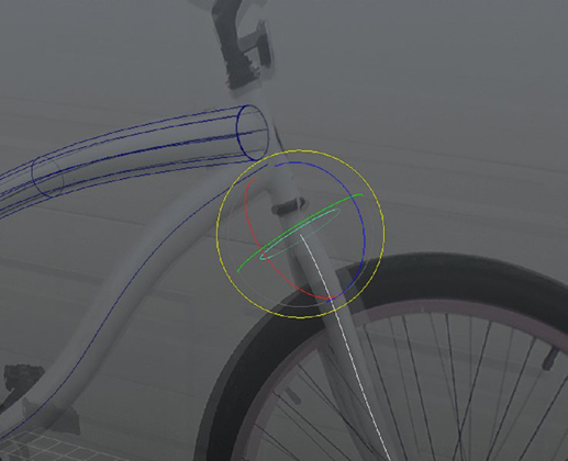
Figure 3.24 Position a new NURBS circle at the top of the fork curve.

Figure 3.25 Extrude the fork for the front tire.

Figure 3.26 The extruded surface is shearing as a result of changing the position of the U CV.

Figure 3.27 The orientation of the NURBS circle has been corrected, eliminating any shearing.

Figure 3.28 Pinching can occur around areas with a high degree of curvature.

Figure 3.29 The number of spans in the construction curve was rebuilt from six to eight.
To see a version of the scene to this point, open the bicycle_v02.ma scene from the chapter3scenes directory at the book’s web page.
Lofting Surfaces
A loft creates a surface across two or more selected curves. It’s a great tool for filling gaps between surfaces or developing a new surface from a series of curves. In this section, you’ll create the bicycle seat from a series of curves.
- Continue with the scene from the previous section, or open the
bicycle_v02.mascene from thechapter3scenesdirectory at the book’s web page. - Create a free image plane using the
seat.jpgfile from thechapter3sourceimagesdirectory at the book’s web page. Transform the image plane roughly to match the scale and position of the seat in the front image plane. Use Figure 3.30 as a guide. -
Starting a lofted surface from scratch can be daunting at first. The trick is not to worry about matching the shape. Instead, create a series of curves, loft the surface, and, through construction history, match the shape.
Looking at the shape of the seat, you can estimate that you will need about eight control vertices to define the seat’s contours. Choose Create ➣ Curve Tools ➣ CV Curve Tool. Make sure that you are using a curve degree of 3. From the front viewport, draw a curve with eight CVs around the thickest part of the seat. Starting at the thickest point ensures that you will have enough CVs to define the surface accurately (see Figure 3.31).
- Using multiple viewports, shape the curve roughly to match the outline of the seat. You are not going for accuracy. You just want to give the curve some shape in all three axes. Eventually, you will mirror the geometry since the seat is symmetrical. Therefore, the curve can start along the center line of the seat or on the XY plane. Also, plan on leaving the bottom open. Use Figure 3.32 as a guide.
- With the curve selected, choose Edit ➣ Duplicate (or press
Ctrl/Cmd+d) to make a standard duplicate of the curve. - Move the curve a unit in either direction.
-
Scaling the curve is a quick way to match the contour of the seat shape. The most effective way to scale the curve and maintain its position along the center line is to move the curve’s pivot point to its start.
Hold
Don the keyboard to enter pivot mode, and holdCto activate Snap To Curve. MMB-click the curve, and drag the pivot point to the start of the curve. Translate the curve to the top of the seat. Scale the curve in the y- and z-axes to match the height and width of the bicycle seat. -
Repeat steps 5 through 7 to get a total of eight curves (see Figure 3.33).
Leave the back of the seat open. It will be easier to close at a later time. Rotate the curve for the front of the seat 90 degrees.
- Select the curves from front to back. The selection order dictates the direction of the surface as well as the lofting order. Selecting curves out of order will result in a loft that overlaps itself.
- Choose Surfaces ➣ Loft ➣ ❒. In the Loft Options dialog box, make sure that the degree of the loft is set to Cubic.
- Click the Loft button. Figure 3.34 shows the lofted surface.
- With the basic surface created, you can now select individual curves and modify the shape interactively. To facilitate shaping the curves, add the surface to a referenced layer. You can also select all of the curves and press F8 to enter Global Component mode (see Figure 3.35). Global Component mode allows you to adjust the components of every object that you select instead of on a per-model basis.
- Name the new surface
seat. When you’re happy with the result, save the model asbicycle_v03.ma.

Figure 3.30 Add a new image plane to use as reference for the seat.

Figure 3.31 Draw a curve at the thickest part of the seat.

Figure 3.32 Shape the curve loosely to match the bike seat.

Figure 3.33 Transform the curves to match the reference images.

Figure 3.34 The duplicated curves are selected in order from right to left, and then a loft surface is created.

Figure 3.35 The CVs of the loft, selected and repositioned to match the reference images
To see a version of the scene to this point, open the bicycle_v03.ma scene from the chapter3scenes directory at the book’s web page.
Attaching Surfaces
Once half of the model is shaped, you can mirror it to the other side and attach the surfaces together. The following steps take you through the process:
- Continue with the scene from the previous section, or open the
bicycle_v03.mascene from thechapter3scenesfolder at the book’s web page. - The construction history is no longer needed. Select the seat and choose Edit ➣ Delete By Type ➣ History.
- Select all of the curves and delete them.
- Select the seat. Choose Edit ➣ Duplicate Special ➣ ❒. Group the duplicate under World, and set Scale to
−1.0in the z-axis (see Figure 3.36). Make sure that the seat’s pivot point is located along the XY plane; you’ll scale from the pivot. Choose Duplicate Special to apply the settings and close the window. - Select the mirrored duplicate and original seat.
- Choose Surfaces ➣ Attach ➣ ❒. You can choose from two different attachment methods. The first, Connect, will attach the two surfaces and preserve the existing shape. Blend will average the control vertices being attached. For the bike seat, choose Blend to create a smooth transition between the two surfaces. Uncheck Keep Originals and click Attach. Figure 3.37 shows the settings.
- The two halves are now one. Notice that the front and back of the surface did not attach. This is because a NURBS surface must have four sides. Delete the node’s history and freeze its transforms.
- You can continue to make adjustments to the surface to match the reference material by modifying its components. There are only two component types that you can manually adjust: hulls and control vertices.
- Save the scene as
bicycle_v04.ma.

Figure 3.36 Use these settings to create a mirror image of the seat.

Figure 3.37 The options for Attach Surfaces
To see a version of the scene to this point, open the bicycle_v04.ma scene from the chapter3scenes directory at the book’s web page.
Converting NURBS Surfaces to Polygons
Today’s production pipelines demand a high degree of flexibility. NURBS excel at creating smooth contours but are not easily combined into complex objects. You can use a NURBS surface to start a polygon model combining the strengths of both NURBS and polygon-modeling tools. You have built multiple pieces of the bike using NURBS surfaces. To take the models to the next level, we’ll convert from NURBS to polygons.
- Continue with the scene from the previous section, or open the
bicycle_v04.mascene from thechapter3scenesfolder at the book’s web page. - Select the bicycle seat.
- Choose Modify ➣ Convert ➣ NURBS To Polygons ➣ ❒.
-
Maya provides numerous tessellation methods for converting NURBS to polygons. For the bike, the best method is going to be control points. Control points work well since we controlled the number of points through the curves used to create the surfaces. Figure 3.38 shows the selected options.
- Converting the bike seat results in a linear polygon surface (see Figure 3.39). It might look as if you wasted your time shaping the model; however, you can enable smooth mesh preview by pressing
3on the keyboard. - Name the new surface
seat. Save the model asbicycle_v05.ma. - Convert the rest of the NURBS surfaces in the scene using the same settings.

Figure 3.38 Convert NURBS To Polygons Options

Figure 3.39 The NURBS surface converted to polygons
To see a version of the scene to this point, open the bicycle_v05.ma scene from the chapter3scenes directory at the book’s web page.
Modeling with Polygons
![]()
![]()
The Modeling Toolkit is the heart of Autodesk Maya’s polygon modeling workflow. For Maya 2016, the toolkit has been integrated to support all of the functionality from within the Move, Rotate, and Scale tools. In addition, the toolkit’s Target Weld Tool is now the default method for merging components. As a result, the Merge Edge and Merge Vertex Tools have been removed. Furthermore, the toolkit has been restructured for better organization.
The polygon tools in general have received a bit of a facelift:
- In-View Editor pop-up menus
- Tools tips within options
- Restructured menus
When dealing with hard-surface objects, you want to stay away from pushing and pulling vertices manually. This generates uneven and inaccurate contours. In general, hard-surface objects are made in factories, where precision is essential to the completion of a product. Modeling can be a numbers game. Aligning parts with the same number of edges/faces makes the modeling process a lot easier. With that, it is beneficial to start a model using primitive objects as opposed to building polygon geometry from scratch. Primitive surfaces provide consistent geometry and can be easily modified through their construction history.
Using Booleans
![]()
A Boolean operation in the context of polygon modeling creates a new surface by adding two surfaces together (union), subtracting one surface from the other (difference), or creating a surface from the overlapping parts of two surfaces (intersection). Figure 3.40 shows the results of the three types of Boolean operations applied to a polygon torus and cube.

Figure 3.40 A polygon torus and cube have been combined using union (left), difference (center), and intersection (right) operations.
Maya 2015 introduced a new carve library for its Boolean operations. The workflow is the same, but the results are improved. Regardless, Booleans are complex operations. The geometry created using Booleans can sometimes produce artifacts in the completed model, so it’s best to keep the geometry as simple as possible. It’s also beneficial to align the edges of one surface with that of another in order to reduce the number of extra divisions that may result.
In this section, you’ll use Boolean operations to weld the different parts of the bike frame together:
- Continue with the scene from the previous section, or open the
bicycle_v05.mascene from thechapter3scenesfolder at the book’s web page. - Select the two largest pipes of the bike frame. The ends of the pipes intersect each other by the handlebars. You can use an intersection to weld these two pipes together. Prior to performing the Boolean operation, the ends need to be cleaned up. Select the end vertices of both pipes (see Figure 3.41).
- Open the options for the Scale tool by double-clicking its icon in the toolbox. The icon is a cube with four red arrows emanating from it.
- Set the Step Snap to Relative and set the Step Size to
1.0. The Scale tool will now snap to a value of 1. - The goal is to make both ends flush with each other and to maintain the angle of the bottom pipe. Change the orientation of the manipulator by matching a point from the lower pipe. Under the Scale Settings rollout, click the triangle next to the xyz coordinate field. Choose Set To Edge. The selection is automatically set to edge in the viewport.
- Select one of the horizontal edges from the top pipe. The manipulator aligns itself to the edge.
- Scale the selection in the x-axis until the vertices are flush with each other. Figure 3.42 shows the result.
- The open edges at either end of the pipes will prevent the Boolean from welding the two objects cleanly. The polygon faces that overlap will remain since neither surface is a closed volume. To close the ends, choose Mesh ➣ Fill Hole.

- You can now use the Boolean tool on the two objects. With both surfaces selected, choose Mesh ➣ Booleans ➣ Intersection. It’s likely that both pipes will disappear after applying the Boolean. From the In-View Editor, choose Edge for the Classification. Figure 3.43 shows the results of the Boolean.
- To bring the fork together with the large pipes of the frame, create a primitive polygon cylinder using the tool’s default settings, Create ➣ Polygon Primitives ➣ Cylinder.
- Position the cylinder to match the reference material. Use the settings in Figure 3.44 to alter the construction history of the cylinder.
- Before intersecting the parts, match up the geometry to avoid overlap and extra divisions. Scaling the ends of the pipe until the vertices reside inside the primitive cylinder works best. Use Figure 3.45 for reference.
- It also helps if additional geometry is added to give the Boolean a better surface to cut into. Select the primitive cylinder, and choose Mesh Tools ➣ Insert Edge Loop.
- Using the default settings of the tool, LMB-click the cylinder at the approximate location where the two frame pipes have been welded together (see Figure 3.46). Release the mouse button when you are happy with the edge loop’s placement.
- Add two more edge loops on either side of the inserted edge loop. Align them with a corresponding edge from the frame. Use Figure 3.47 as a guide.
- Select the frame, fork, and cylinder. The order is irrelevant. Choose Mesh ➣ Booleans ➣ Union. Figure 3.48 shows the result.
- Delete the history, and save your scene as
bicycle_v06.ma.

Figure 3.41 Select the ends of the two largest parts of the bike frame.

Figure 3.42 Scale the ends of the pipe to make them flush with each other.

Figure 3.43 Use Intersection to join the two parts of the frame together.

Figure 3.44 Position and alter the cylinder’s construction history.

Figure 3.45 Scale the ends of the frame pieces to fit inside the primitive cylinder.

Figure 3.46 Insert an edge loop into the cylinder.

Figure 3.47 Insert two more edge loops into the cylinder.

Figure 3.48 Use a union Boolean to weld all three parts together.
To see a version of the scene to this point, open the bicycle_v06.ma scene from the chapter3scenes directory at the book’s web page.
Cleaning Topology
Topology refers to the arrangement of polygon edges on a surface. The versatility of polygons allows you to alter components freely, which can result in bad topology. As a result, the polygons often require a bit of work to maintain their integrity. In this section, we’ll look at multiple tools for adding and removing polygon components.
- Continue with the scene from the previous section, or open the
bicycle_v06.mascene from thechapter3scenesfolder at the book’s web page. - The Boolean applied in the previous section has left numerous n-sided polygons and overlapping edges. You can clean these up quickly with the Target Weld tool. Choose Mesh Tools ➣ Target Weld. RMB-click the geometry and choose Vertex. A red circle shows up around the closest vertex to your mouse as a preselection highlight (see Figure 3.49).
-
The difference between a stray vertex and a vertex with good topology is that a stray vertex does not conform to the existing structure of the geometry. LMB-click a stray vertex, and drag to a vertex with good topology. A line is displayed between the two vertices.
Notice how the good edges define the structure. Eliminating the vertices surrounding them will have little impact on the surface shape.
- Work your way around the frame connection points. Only do one side or half of the geometry. Eventually, the clean side will be mirrored across. Figure 3.50 shows the bicycle frame after the stray vertices have been welded to existing vertices.
-
You can also eliminate the edges that are creating triangles on the surface. Having them gone will make modifying the surface easier and make the surface smoother, especially with smooth mesh preview (see Figure 3.51).
There are two ways that you can delete an edge. The first is simply to select the edge and press Delete on the keyboard. The second is to select the edge and choose Edit Mesh ➣ Delete Edge/Vertex or press Ctrl+Delete. The difference between the two methods is that the latter will delete any non-winged vertices associated to the edge. Go through the area that you cleaned and remove the triangle edges. It should only be necessary to press Delete on the keyboard.
- Use the Boolean tools for the rest of the bike frame and clean the topology. Add more cylinders as needed. Remember, you need to do only one side.

Figure 3.49 A preselection highlight is activated when using the Target Weld tool.

Figure 3.50 The bike frame has been cleaned of stray vertices.

Figure 3.51 The triangle-forming edges have been removed.
To see a version of the scene to this point, open the bicycle_v07.ma scene from the chapter3scenes directory at the book’s web page.
Creating Your Own Polygons
Primitives are a great place to start modeling, but some shapes are too irregular to make with primitives. You can build your own polygon shapes to begin a model. The following section walks you through the process of building the odd-shaped tire hanger of the rear tire.
- Continue with the scene from the previous section, or open the
bicycle_v07.mascene from thechapter3scenesfolder at the book’s web page. Half of the bike frame has been removed for simplicity. - Choose Mesh Tools ➣ Create Polygon.
- Using the tool’s defaults, LMB-click to create the basic shape of the tire hanger. Leave out the round tab at the top-left corner (see Figure 3.52). When finished, press Enter to complete the shape.
- When you’re building a round shape from scratch, there is no need to try to draw a circle. Instead, start with a primitive object, like a cylinder or sphere, to get a rounded object. You can then integrate the rounded shape into your object. For the tab, create a primitive cylinder.
- Transform the cylinder to match the size and location of the screw hole in the tab. Use Figure 3.53 as a reference.
- Select all of the faces of the cylinder except for one end. Press Delete to remove the geometry, leaving a polygonal disc (see Figure 3.54).
- With the disc selected, choose Modify ➣ Center Pivot. The pivot point is forced into the middle of the disc.
- Snap the disc to the XY grid plane. You can use the hot key
xto snap to grid. - To complete the tab, RMB-click the geometry and select Edge. Double-click any of the exterior edges to select the entire outer loop.
- Choose Edit Mesh ➣ Extrude. Extrude the edge selection to match the outer size of the metal tab (see Figure 3.55).
- Delete the faces for half of the disc. Do not include any of the faces on the interior circle.
- Select the border edges from the side of the disc that you deleted. You can select the row of edges by clicking the first edge and then double-clicking the last.
- Choose Extrude. Do not move the extrusion. Choose the Move tool, and open its tool options. You want to translate the newly extruded edges in a linear direction that matches the center line of the disc. To do this, expand the Transform Constraint option menu and select Set To Edge from under the Move tool settings. Click the center edge. The Move tool updates to the new orientation.
- Translate the edge selection to where it meets the polygon edge of the tire hanger, as shown in Figure 3.56.
- Open the Scale tool options. Set the orientation of the Scale tool to the same edge from step 13. Scale the edge selection with a discrete scale of
1.0to make the edges coplanar. Figure 3.57 shows the result. - You can now delete the interior faces that make up the hole of the tab. To select the faces quickly, RMB-click the geometry and choose Vertex. Click the center vertex of the interior disc. Ctrl+RMB-click the geometry and, from the marking menu, choose To Faces ➣ To Faces. Delete the selected faces.

Figure 3.52 Use the Create Polygon tool to draw a custom shape.

Figure 3.53 Position a primitive cylinder in the screw hole of the tab.

Figure 3.54 Delete the faces of a cylinder to create a disc.

Figure 3.55 Extrude the edges of the polygon disc.

Figure 3.56 Translate the edges in the x-axis to meet the edge of the tire hanger.

Figure 3.57 Scale the edges to make them coplanar.
To see a version of the scene to this point, open the bicycle_v08.ma scene from the chapter3scenes directory at the book’s web page.
Multi-Cut Tool
![]()
The Multi-Cut tool allows you to divide polygon faces. You can use it to make simple divisions, from one vertex to another, or to cut through multiple edges all at once. You are also allowed to draw divisions inside existing faces as long as you end up on an adjacent edge. The Multi-Cut tool effectively replaces the Interactive Split Polygon tool and the Cut Faces tool, and with the use of Ctrl and the Modeling Toolkit, you can also eliminate the Insert Edge Loop tool. To see the Multi-Cut tool’s fullest potential, watch MultiCut.mov in the chapter3movies folder at the book’s web page. Figure 3.58 shows an example of the Multi-Cut tool in action.

Figure 3.58 With the Multi-Cut tool, you can draw divisions inside existing faces.
The following steps walk you through adding divisions with the Multi-Cut tool:
- Continue with the scene from the previous section, or open the
bicycle_v08.mascene from thechapter3scenesfolder at the book’s web page. - The tab and custom polygon shape need to be merged together. Before you can do this, their components must match. Select the custom polygon shape.
- Choose Mesh Tools ➣ Multi-Cut. LMB-click the inside loop and then the outside edge to create a division. RMB-click to complete the division. You can also press Enter to complete the cut. Use Figure 3.59 as a guide.
- Continue to add divisions to the surface. You need enough divisions, around six, to create a circular shape. The tire hanger has two circular shapes: one on the inside and one on the outside. Use the Multi-Cut tool to connect the two half-circles (see Figure 3.60).
- Use the Multi-Cut tool to remove the remaining n-gons on the surface. You can click and hold an edge to drag the division along the length of the edge to be divided. Holding Shift snaps the division to 10-percent increments. Figure 3.61 shows the new divisions.

Figure 3.59 Use the Multi-Cut tool to add a division to the custom polygon shape.

Figure 3.60 Add divisions to round out the interior and exterior of the tire hanger.

Figure 3.61 Divide the geometry to get rid of any n-gons.
To see a version of the scene to this point, open the bicycle_v09.ma scene from the chapter3scenes directory at the book’s web page.
Combining and Merging Geometry
Typically it’s best to build complex parts as individual pieces and then bring them all together to form a single object. The tire hanger is made up of two separate pieces. To join them into one, you will use a combination of tools. The following steps take you through the process:
- Continue with the scene from the previous section, or open the
bicycle_v09.mascene from thechapter3scenesfolder at the book’s web page. - Select the tab and custom polygon shape. Choose Mesh ➣ Combine. The two separate objects are now a single node.
-
Delete the node’s history, and rename the node to
tireHanger. - Select the four vertices that make up the center of the tab and polygon shape (see Figure 3.62).
- Choose Edit Mesh ➣ Merge To Center.
- Select the remaining vertices on one side of the tab. Use Target Weld to drag the entire selection to the left corner vertex of the custom polygon shape. Figure 3.63 shows the end result.
- Repeat step 6 for the other side of the tab shape.
- Shape the geometry to match the reference material. Save your scene as
bicycle_v10.ma.

Figure 3.62 Select the middle vertices by the connection point of the combined object.

Figure 3.63 Weld half of the vertices to a single vertex.
To see a version of the scene to this point, open the bicycle_v10.ma scene from the chapter3scenes directory at the book’s web page.
Bridge Polygon
The Bridge tool appends a series of polygons between border edges. The border edges must reside on the same node before the Bridge tool will work. The Bridge tool can make quick work of connecting the tire hanger to the frame of the bike. To use the Bridge tool, follow these steps:
- Continue with the scene from the previous section, or open the
bicycle_v10.mascene from thechapter3scenesfolder at the book’s web page. - Select the tire hanger. Extrude the geometry in the local z-axis to 0.1.
- Center the object’s pivot. Snap the object to the center line of the frame, as Figure 3.64 shows.
- To bridge between two objects, the border edges that you want to bridge must have the same number of edges. With the tireHanger node selected, choose Mesh Tools ➣ Multi-Cut ➣ ❒. The Modeling Toolkit opens.
- Hold Ctrl and MMB-drag any edge along the thickness of the tire hanger (see Figure 3.65). The MMB forces the edge loop to be snapped along the center of the chosen edge. Release the mouse button to insert the loop.
-
Select the four faces next to the lowest bar on the bike frame and delete them. This creates a border edge. Use Figure 3.66 for reference.
- Select the frame and tire hanger. Combine the objects into a single node.
- RMB-click the object, and choose Edge from the marking menu.
- Double-click both border edges, as shown in Figure 3.67.
- Choose Edit Mesh ➣ Bridge. The defaults create too much geometry. In the In-View Editor menu, change Divisions to
1(see Figure 3.68). - Repeat the steps 5 through 9, omitting step 6, to bridge the upper part of the bike frame. Figure 3.69 shows the finished product. Save your scene as
bicycle_v11.ma.

Figure 3.64 Snap the tire hanger to the center line of the bike frame.

Figure 3.65 Insert an edge loop down the middle of the thickness of the tire hanger.

Figure 3.66 Delete the four faces closest to the lower bar of the bike frame.

Figure 3.67 Select the border edges.

Figure 3.68 Change the number of divisions in the bridge to 1.

Figure 3.69 Bridge the top section of the frame.
To see a version of the scene to this point, open the bicycle_v11.ma scene from the chapter3scenes directory at the book’s web page.
Mirror Cut
The Mirror Cut tool creates symmetry in a model across a specified axis. The tool creates a cutting plane. Any geometry on one side of the plane is duplicated onto the other side and simultaneously merged with the original geometry.
In the options for Mirror Cut, you can raise the Tolerance, which will help prevent extra vertices from being created along the center line of the model. If you raise it too high, the vertices near the center may collapse. You may have to experiment to find the right setting.
- Continue with the scene from the previous section, or open the
bicycle_v11.mascene from thechapter3scenesdirectory at the book’s web page. - Select the bike frame, and choose Mesh ➣ Mirror Cut ➣ ❒. Set Cut Along to the XY plane and choose Mirror Cut. A plane appears down the center of the bike frame’s geometry.
-
Set the Translate Z channel of mirrorCutPlane1 to
0.0. The mirrored geometry is extended.In the Outliner, several new nodes have been created. These include the mirrorCutPlane1 and the mirroredCutMesh1 group. The frame has been renamed to polySurface18 (see Figure 3.70).
- Select the polySurface18 node, and choose Edit ➣ Delete By Type ➣ History. This removes the group nodes that were created. Select the mirrorCutPlane1 node, and delete it.
- Name the polySurface18 node
frame.

Figure 3.70 Mirror the frame across the z-axis using the Mirror Cut tool.
To see a version of the scene to this point, open the bicycle_v12.ma scene from the chapter3scenes directory at the book’s web page.
The rest of the bike can be modeled using the methods and techniques outlined in this chapter. When approaching a new piece, ask yourself if there is a primitive object that closely matches the surface shape or even a portion of the surface shape. For instance, the bike tire can be created quickly using a primitive polygon torus. You can use the following settings for the torus’s construction history.
- Radius:
6.21 - Section Radius:
0.52 - Subdivisions Axis:
30 - Subdivisions Height:
8
Figure 3.71 shows the finished version of the bike. You can also open the bicycle_final.ma scene from the chapter3scenes directory at the book’s web page.

Figure 3.71 The finished version of the bicycle
The Bottom Line
Understand polygon geometry. Polygon geometry consists of flat faces connected and shaped to form three-dimensional objects. You can edit the geometry by transforming the vertices, edges, and faces that make up the surface of the model.
Master It Examine the polygon primitives in the Create ➣ Polygon Primitives menu.
Understand NURBS surfaces. NURBS surfaces can be created by lofting a surface across a series of curves. The curve and surface degree and parameterization affect the shape of the resulting surface.
Master It What is the difference between a one-degree (linear) surface, a three-degree (cubic) surface, and a five-degree surface?
Understand subdivision surfaces. Any polygon object can be converted to a subdivision surface directly from its Attribute Editor. Maya offers three different methods for subdivision.
Master It Convert a polygon model to a subdivision surface model. Examine how the polygon object changes in shape.
Employ image planes. Image planes can be used to position images for use as a modeling guide.
Master It Create image planes for side, front, and top views for use as a model guide.
Model with NURBS surfaces. A variety of tools and techniques can be used to model surfaces with NURBS. Hard-surface/mechanical objects are well-suited subjects for NURBS surfaces.
Master It Create the spokes of the bike.
Model with polygons. Booleans can be a great way to cut holes quickly into polygon surfaces. It is important, however, to establish a clean surface for the Boolean to cut into or intersect with. When you’re using multiple objects, doing so becomes even more important.
Master It Create the hub to which all of the bicycle spokes will attach. Each spoke should have its own hole.