Chapter 7
Working with Different Costs and Cost Curves
In This Chapter
![]() Learning two different views of costs
Learning two different views of costs
![]() Distinguishing average, total, and marginal costs
Distinguishing average, total, and marginal costs
![]() Connecting costs to staying in business
Connecting costs to staying in business
Much of the production in an economy comes from firms. In a market-based economy, these firms make their decisions based on an indicator, profit, which expresses the difference between the revenues the firm takes in and the costs it expends in obtaining those revenues. To understand how a firm makes such decisions, as well as how economists look at them, you need to examine more closely the relationship between the different types of cost a firm faces — what economists call its cost structure.
In a market economy, and certainly in an economically liberal society, a firm can’t simply march people to its showrooms, lock the doors, and force them to buy its product, much as they might like to. So, although a firm may know a lot about how to organize production or how to produce, it doesn’t necessarily know how much a consumer will want to buy at a given price — at least until it starts to get data from transactions. And it certainly can’t control how much people will buy at that price (though it may have a good basis for guessing). Therefore, economists look at the aspects of a firm’s operations that it does control, which means looking seriously and carefully at its costs.
This chapter examines a firm through its cost curves, which provide a relationship between a given cost incurred to produce and how much a firm will produce for that cost. We define and then investigate a firm’s total, marginal, and average costs, see how they interact within a firm, and discuss their importance in firms surviving and continuing to trade or going under.
Understanding Why Accountants and Economists View Costs Differently
Economists look at costs in a particular way, which may not be what you expect. Every firm in every industry in every country incurs costs of one kind or another, and accounting systems provide a way of measuring and recording them. But economists are interested in more than the record of what was done in the past. They also want to know what opportunities the firm did not pursue or what the firm could have done had it not made the decision it did. Therefore, economists tend to look at costs in a different way.
In a set of company accounts, you find many items that describe costs, from costs of goods sold to overheads to general expenditures (these are accounting costs). Company accounts are produced to a set of standards that reflect the accounting profession’s view of how best to describe the costs of a company, given that those costs are incurred in different ways and at different stages of production. As a result, companies report many different cost measures, and accountants know how to interpret these measures as needed.
 Economists treat costs in a slightly different way, called, unsurprisingly, economic costs. Whereas an accountant needs to know what costs have accrued over the past year, an economist wants to examine costs as they relate to the firm’s decision-making. This involves some key subtleties, the most important of which is that economic costs account for the opportunities the firm had to give up in order to do what it’s doing. Economists call these opportunity costs. In principle, a firm has to account for them before going on to make any decisions about production or investment so that it knows it’s making the decision on a rational basis.
If you’re scratching your head a little, here’s an example to relieve that itch.
Suppose you gave up a decently paying job to start a business and at the end of your financial year your accountant sends you a statement saying that your revenue was in excess of your costs by $25,000. You’re happy with this, considering that an accounting profit of $25,000 is a decent return on your business. But then your economist friend points out that the job you gave up was paying a net salary of $35,000, which means that you gave up an opportunity to make $10,000 more than you received from your new business.
 In fact, your accounting profit of $25,000 was an economic loss of $10,000 when you factor in the opportunity cost of giving up your old job to start your business. (Economics is called the dismal science for a reason.)
The upshot is that when looking at the individual types of cost a firm incurs, you can assume that economists (and this book) are talking about economic costs that include opportunity costs.
Looking at a Firm’s Cost Structure
When considering a firm, economists place emphasis on its cost structure, which means looking at the different ways to break down or measure costs, depending on the parts of the picture they’re looking at.
Typically microeconomists use three different ways to express the costs of a firm:
- Total cost looks at total cost for a given level of production.
- Average cost looks at how much producing a given level of output will cost per unit of output.
- Marginal cost looks at how much costs increase to produce an additional unit of output.
Economists also tend to break down costs according to the planning horizon or period of the firm and use these relationships to discover something about the structure of a firm or the technology of production it engages in:
- Fixed costs do not vary for the planning horizon considered. These costs are fixed and do not depend on the size of output.
- Variable costs vary for the planning horizon considered and depend on the size of output.
Taking in the big picture: Total costs
When talking about the types of cost a firm faces, economists start with the biggest and least detailed view of costs and then break them down in ways that make sense for economic decision-making.
The most global view of a company is in terms of its total costs (TC), which economists use quite simply to arrive at a number for total profits (you don’t need to worry about gross or net terms here). Total costs are simply the overall cost of making a product and serving it to a market after all those relevant cost elements are accounted for.
If you start with a number for total revenue received (TR) and then subtract all those costs, you arrive at a figure for profit. We write that as an equation here:
![]()
 The Greek symbol Π in the equation stands for profit, so that economists don’t get confused with price (generally denoted with a P).
When you take the view of firm owner, you may want to start looking at aspects of the total cost a little more closely. The simplest way to break down total costs is into two categories:
- Costs that depend on the amount you’ve produced: These include all things that are ongoing in the sense that the more you produce — or for a service, the more activity you undergo — the more you pay, which means things such as costs of each input used or the cost of utilities. These are called variable costs, and economists usually denote them VC when talking about variable costs as a component of total costs.
- Costs that don’t depend on the amount you’ve produced: These include all the elements that your firm would have to pay regardless of how many items it produces. These may be the cost of premises, such as rents, or licenses if needed, or even the cost of advertising that the firm has to buy to let people know about its business. Economists call these fixed costs and usually abbreviate them FC.
Together, the two types of cost must sum to the total cost at which the firm operates, so we can say:
![]()
Here’s an example: A bicycle manufacturer makes bikes using labor, materials, and utilities costing $10 a bike. Assuming that she makes 100 bikes in a production period, the variable costs (VC) she faces will be 100 bikes times $10 a bike, which equals $1,000. However, in order to do this she needs a factory with the capacity to make the bikes: That factory costs $10,000 to rent per period. So her total costs are fixed costs (FC) of $10,000 plus the VC of $1,000, which equals $11,000 total costs.
Here are two important points to bear in mind:
- You have to pay fixed costs even if you produce absolutely no output whatsoever. If, for instance, you take out a rental contract for an office, you have to pay the rent irrespective of whether you produce anything at all.
- Variable costs depend on the amount of output you produce. If you have a pizza restaurant and you make no pizzas, you don’t need any flour, tomatoes, or even power for a pizza oven. But the more pizzas you make, the more you spend on these inputs.
Measuring by unit: Average costs
By itself, total cost doesn’t say much about the firm and still less about how it makes its decisions. Economists want to discover a little more about how the firm operates, so they look at the relationship between total cost and the number of units produced. To do so, they divide the cost of production by the number of units produced to derive the average costs.
Making use of average costs
Average costs or the cost per unit, measured at a level of production, are useful things to know in and of themselves, but they also have some important properties that economists use to find out about the efficiency of production. To compute average total cost (ATC), you divide total costs (TC) by the quantity produced (Q):
![]()
Now, here’s an interesting thing. As already mentioned, total costs break down into fixed costs (FC) and variable costs (VC). Therefore you can divide each of these components by quantity of output produced to get average fixed costs (AFC) and average variable costs (AVC), which are the amount of fixed cost per unit and the amount of variable cost per unit, respectively. Or to put it another way:
![]()
To discover an interesting feature of a firm’s costs of production, take a look at average fixed costs. Fixed costs don’t change whatever the level of production, but as you go on producing more and more, the AFC per unit falls as you divide by a higher level of output each time.
Here’s a very simple example: A baker needs to incur a cost of $100 to set up his premises and can then make cakes for $2 per cake. The total cost is the sum of fixed and variable costs. Let Q denote the number of cakes produced. This allows us to write the following formula for his total costs:
![]()
Now divide through by quantity of cakes produced to get average total cost:
![]()
We now plot some numbers for the average total cost (ATC), or more simply (AC). Table 7-1 computes total and average costs according to this formula.
Table 7-1 Relationship between Total, Average, Fixed, and Variable Costs
|
Quantity Produced |
1 |
2 |
3 |
4 |
5 |
6 |
|
Fixed cost |
100 |
100 |
100 |
100 |
100 |
100 |
|
Variable cost |
2 |
4 |
6 |
8 |
10 |
12 |
|
Total cost |
102 |
104 |
106 |
108 |
110 |
112 |
|
Average total cost |
102 |
52 |
35.333 |
27 |
22 |
18.667 |
|
Average fixed cost |
100 |
50 |
33.333 |
25 |
20 |
16.667 |
|
Average variable cost |
2 |
2 |
2 |
2 |
2 |
2 |
Take a look at the average total cost row. If you notice that it falls as we add more units, that’s good. Now look at the next two lines, the costs broken down into fixed and variable components. Note that the average fixed costs are particularly falling. Why? Well, a fixed cost doesn’t depend on how much a firm produces — it still has to pay the same cost. In this case, though, because it’s making more units, the fixed cost is being divided by more units each time, which means that as the firm makes more, the average fixed cost gets smaller.
 This fact is a key principle behind the concept of economies of scale. As the baker produces more cakes, he does so for a lower cost per cake.
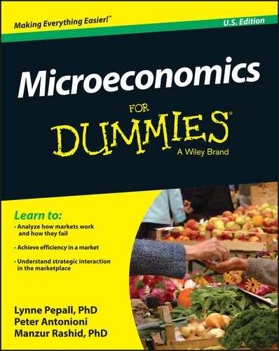
Visualizing economies of scale by plotting average costs
One way to see how this works is to plot the average cost over a range of production. Generally the average cost curve is U-shaped. Over the range of output, as more gets made, the fixed costs get spread out over more output and average costs fall. Average costs stop falling when the increase in average variable costs in expanding production outweighs the decrease in average fixed costs. This does not happen in Table 7-1’s example because average variable costs are constant and do not go up as production increases.
Average costs typically fall up to a point, beyond which the increase in average variable costs from adding an extra unit is greater than the decrease in average fixed costs by adding an extra unit. At this point, economists say that the firm has fully exploited economies of scale and is experiencing diseconomies of scale.
Figure 7-1 shows that average fixed cost is always falling, because the same number is divided by a bigger number each time, but that average variable costs start to rise beyond a certain point. That point, where the average cost of production rises again, is the minimum efficient scale of production and is important for considering the efficiency of a firm. Just note it for the moment: we say more about what efficiency means in this context in Chapter 8.

© John Wiley & Sons, Inc.
Figure 7-1: Average costs, average variable costs, and average fixed costs for a typical firm.
Adding only the cost of the last unit: Marginal cost
The breakdowns used in the preceding sections show costs for a particular level of production. But economists also use another important measure to consider when considering a firm’s costs: marginal cost.
Meeting marginal cost
Put simply, marginal cost (MC) is the cost of adding one extra unit of output to your current output level. (A unit of output could be a ton of steel, a cake, a bushel of wheat, an hour of dental cleaning services, all depending on the output and the units of measurement.) Imagine that you produce 10 beach balls for $10 in total cost. If you add an extra beach ball to your production and make the total cost $11, the marginal cost of the 11th beach ball is $1, because that’s how much producing an extra beach ball adds to your total costs.
Economists express marginal costs in terms of the change in total costs, which means that they measure a change in total cost for a change in quantity. Thus marginal costs are a measure not of how much something costs but how much those costs are changing as you do something to production.
“Marginal anything” in economics is important, because it is often the case that decision-making occurs at the margin. If you are already doing something, say making 100 units, and have already made that decision, then you must decide whether to make the 101st unit. That’s the marginal decision you face.
You can calculate MC fairly simply, even across a number of units by remembering that it’s the change in cost for a small change in quantity (Q). So, quite simply taking the change in total cost (TC) and dividing by the change in quantity gives you an answer:
![]()
Tracking where MC crosses the AVC and ATC curves
Marginal cost curves always cross the average variable and average total cost curves at the minimum of those curves — that is, at the bottom of the U-shapes that make up both curves. (Average fixed costs are different: they can fall over the whole of the production range and therefore not have a bottom of the U). This intersection has to happen because marginal costs capture the change in costs that determines whether or not average variable or average total costs are rising or falling.
To see why, let’s move away from costs and think about worms for a while. Suppose a biologist is working out the average length of wiggly worms in a sample. Suppose she’s measured 10 of them and come up with an average length of 5 inches. Now imagine that she’s given an 11th sample. If the 11th worm is longer than 5 inches, the average length of the worms in her sample goes up. If it’s less than 5 inches, of course, the average in the sample goes down. But if the marginal worm is exactly 5 inches long, the average stays at exactly 5 inches.
Back to costs. Suppose the average cost of producing ten units is $1. If the cost of adding an extra unit is greater than $1, the total cost of producing all the units is more than $11, and the average cost of production is more than $1. But suppose that the marginal cost of an extra unit is 90 cents. Then the total cost is $10.90 and average cost is 99 cents — average cost has fallen. On the other hand, if the marginal cost is exactly $1, average cost is also exactly $1.
So we have three cases:
- Average cost falls when the marginal cost of producing an extra unit is less than the average cost of producing all previous units.
- Average cost rises when the marginal cost of the extra unit is greater than the average cost of producing all preceding units.
- Average cost stays the same when the marginal cost of producing an extra unit is exactly the same as the average cost of producing the previous units.
You can see this effect illustrated graphically in Figure 7-2. These “typical” average curves are split at their minimum points (bottom of the U) by a marginal cost curve.

John Wiley & Sons, Inc.
Figure 7-2: Relationship between average (AC) and marginal cost (MC). AVC = average variable costs.
Here’s a key implication. To minimize costs, you want to be at the minimum of the average total cost curve (i.e. the minimum of AC in Figure 7-2). You’re at that point when the marginal cost of adding an extra unit of production is exactly the same as the average costs of all the preceding units. So, to produce for the lowest possible cost, you know not to produce when the marginal cost is greater than average cost, and that if your marginal cost curve is below average cost, you’re better off in terms of average cost when you expand your production up to the point where they’re equal.
Putting it together: Cost structure of a simple firm
This section considers a simple firm example to show how microeconomics looks at the cost structure of firms in general.
Zio Enzo’s Pizza makes authentic Italian-style pizzas and is considering how to minimize its costs. Enzo asks his daughter, Maura, to use her first-year microeconomics training to look at the firm’s cost structure. She deduces the following:
- Fixed costs will be $100 per week, no matter how many pizzas are produced.
- A pizza-maker is paid $10 per hour for an 8-hour day, or $80 per day.
- Enzo’s has no variable costs other than the labor that goes into making them (implausibly, out of all the pizzerias in the world!).
- The variable cost that’s relevant is the number of pizza-makers employed to produce the firm’s output.
- The output initially improves as the firm hires more pizza-makers, because two can produce more output than one. But soon enough a bench full of pizza-makers start getting in each other’s way as they fling dough around, and this reduces the net contribution of each successive pizza-maker.
Maura collects all the data together and summarizes it (see Table 7-2).
Table 7-2 Cost Structure of Zio Enzo’s
|
L |
Q |
Q/L |
FC |
AFC |
VC |
AVC |
TC |
ATC |
MC |
|
0 |
0 |
- |
100 |
- |
0 |
- |
100 |
- |
- |
|
1 |
50 |
50 |
100 |
2 |
80 |
1.6 |
180 |
3.6 |
1.6 |
|
2 |
140 |
70 |
100 |
.71 |
160 |
1.14 |
260 |
1.86 |
.89 |
|
3 |
220 |
73.3 |
100 |
.45 |
240 |
1.09 |
340 |
1.55 |
1.00 |
|
4 |
290 |
72.5 |
100 |
.34 |
320 |
1.10 |
420 |
1.45 |
1.14 |
|
5 |
350 |
70 |
100 |
.29 |
400 |
1.14 |
500 |
1.43 |
1.33 |
|
6 |
400 |
66.7 |
100 |
.25 |
480 |
1.20 |
580 |
1.45 |
1.6 |
|
7 |
440 |
62.9 |
100 |
.23 |
560 |
1.27 |
660 |
1.50 |
2 |
|
8 |
470 |
58.8 |
100 |
.21 |
640 |
1.36 |
740 |
1.57 |
2.7 |
L = Labor (number of workers), Q = Quantity (output), Q/L = Output per worker, FC = Fixed cost, AFC = Average fixed cost, VC = Variable cost, AVC = Average variable cost, TC = Total cost, ATC = Average total cost, MC = Marginal cost
Here’s what Maura can tell about the business from this breakdown of the cost structure. From the output per worker column she notices an interesting, but entirely normal phenomenon: more gain in output comes from adding the first incremental worker than from adding the eighth. As she suspected, the firm gains increasing returns from the first additional pizza-maker joining the team. But after adding the third, they start to get in each other’s way, making their additional contribution to output decrease. The more workers she adds, the smaller their contribution to output becomes.
Economists call this a case of diminishing returns which occurs when adding additional increments of labor to a production premise or plant of fixed size.
Now let’s plot the data points for average and marginal costs in Figure 7-3.

© John Wiley & Sons, Inc.
Figure 7-3: Cost curves for Zio Enzo’s.
Although both average cost curves are shallow (because of the low numbers of workers relative to the number of pizzas produced), they are, more or less, the U-shaped curves mentioned in the earlier section “Tracking where MC crosses the AVC and ATC curves.” Also note that the marginal cost curve goes through both of those minimum points.
Applying microeconomic thinking to the cost-minimizing level of production, Maura can tell her father that he makes himself best off at the point where he’s employing three pizza-makers to do the work. (Clue: The lowest average variable cost of making pizzas is, as you can see from Table 7-2, at three workers. When you increase the number of pizza-makers by one, the marginal cost added is greater than the average variable cost, and so you can see that you’ve passed the sweet spot and costs are now increasing again.)
Relating Cost Structure to Profits
The motivation for a firm staying in business is that its revenues exceed its costs (including opportunity costs — see the earlier section “Understanding Why Accountants and Economists View Costs Differently” for a definition). When revenues exceed costs, the firm is making profits. Therefore, we need to consider a firm’s revenue side. This section introduces the ideas of profit maximization and shutdown conditions.
Looking at firm revenue
How much a firm produces — or whether it produces at all — also depends on how much revenue a firm takes in. The firm can control its costs better than it can control its revenue, but it still needs to be taking in money in some way, or it is unlikely to remain a business for very long. Because profits are the difference between revenues generated and costs expended, you have to know something about how the firm’s revenue relates to its costs to know something about profits. So, in this section, we show you how to manipulate revenue equations to see how much profit a firm might make, and when not making anything and shutting down is the wisest option.
We begin by extending the example of Zio Enzo’s Pizza from the preceding section. We make a simple and probably ridiculous assumption that Enzo’s is a price taker (check out Chapter 10 for more on price takers and their opposite, price makers). Being a price taker means, quite simply, that Enzo’s has no influence on the price that the market is willing to pay for the delicious, imaginary pizzas that Enzo makes. Instead we assume that the market is willing, in general, to pay $2 a pizza (it must be in a student area), and that no relationship exists between Enzo and any competitors.
Remember the formula to work out profits:
![]()
Now we take the term for total revenue and expand it. Total revenue (TR) received for selling Q units of a product at price P is:
![]()
So how can the firm discover whether total revenue is greater than total costs, and if so by how much? Here’s a trick: Average total cost (ATC) is TC divided by Q, and so ATC multiplied by Q will give you TC. Therefore:
![]()
The two terms for revenue and costs contain Q, and so we divide both sides by Q to drop it out.
Let’s focus on the two terms on the right-hand side of the equation. If P (the price a firm receives for its output) is greater than average total cost, the firm supplying that good makes economic profits greater than zero. If the price is less than average total cost, the firm is taking losses. When the two are equal, revenues are equal to economic costs, and the firm makes economic profits of zero.
The optimal condition for how much output a firm should be willing to supply (the best that it can possibly do given its costs and revenues) is satisfied when the marginal cost (MC) of producing an extra unit is equal to the marginal revenue (MR) received from selling it.
Hitting the sweet spot: When MC = MR
When the marginal revenue gained from an extra sale is equal to the marginal cost incurred in making the good, the firm is maximizing its profits. Put another way, if supplying an extra unit costs more than the firm receives by selling it, the firm is better off not doing it. If supplying an extra unit costs less than the firm receives from selling it, the firm is better off producing it.
When making a decision, the firm is interested only in the last incremental unit of the product, whether you’re talking about revenues or costs. All previous production is irrelevant: The firm just needs to focus on whether to make the last unit and, given that, whether producing the unit yields a profit.
Figure 7-4 adds a new line (compared to Figure 7-3) for the marginal revenue gained from selling an extra pizza. The assumption made in the preceding section — Enzo’s is a price taker — means that in this case, marginal revenue is a horizontal line at a price of $2.

© John Wiley & Sons, Inc.
Figure 7-4: Optimal production decision for Zio Enzo’s.
Notice that the marginal cost line crosses this line when MC = MR, which is exactly at 440 pizzas. So, Enzo’s will be making the optimal production decision where it produces 440 pizzas — where exactly as much is yielded from selling one more pizza as it costs to make.
This concept is so important that we now think about it in another way. Look back at Table 7-2 and notice that the marginal cost of all the pizzas before the 440th is less than $2. Now look at the 400th pizza, which Enzo can make for a marginal cost of $1.60. If he were to make 400 pizzas, the marginal pizza would yield revenue of $2 but have a cost of only $1.60, which, you’d suppose, would make for one happy Enzo.
But Enzo could even be made happier by selling pizzas numbers 401 to 440. He would be better off in terms of making more money by expanding his production to the level where the cost of producing the last pizza and the benefit or revenue from selling it are equal. On the other hand, if he were paying more than $2 to make a pizza that only yields $2, he’d be better off reducing his output until the two were equal.
The very best production decision a firm can make is when MC = MR.
Viewing profits and losses
Here are two observations concerning profits and losses for a firm under the condition of producing optimally:
-
Finding Q* where MC = MR allows the firm to make the optimal output.
- At Q* (the optimal amount of production), the firm isn’t guaranteed a positive profit, but this is the point at which it maximizes profit (and if it must take losses, this output minimizes losses).
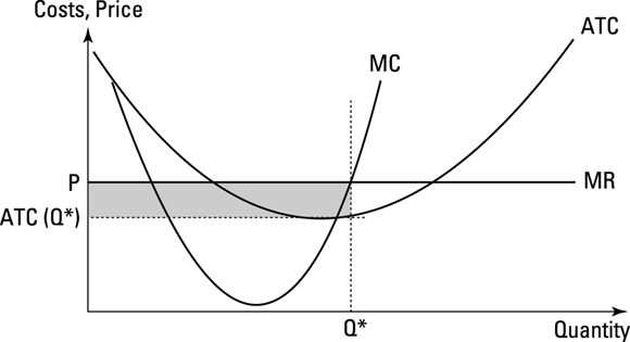
We now walk you through understanding whether a firm will or won’t make a profit in a very simple way. Figure 7-5 shows the costs and output for a generic company (we’re not using the specific numbers as we did for Zio Enzo’s). The optimal output (where MC = MR) is indicated with Q*. Now at Q*, price is greater than average total costs.
© John Wiley & Sons, Inc.
ATC = Average total cost, MC = Marginal cost, MR = Marginal revenue, Q* = Optimal amount of production, P = price
Figure 7-5: Profits for a price-taking firm when P > ATC.
At this point you can use a little sleight of hand to show profits: Remember that revenue is simply price times quantity. On our mapping of price and quantity that’s also the area of a rectangle bounded by the axes, the MR line, and Q*. Then move on to the total cost, which is going to be ATC times Q* — that is, the average total cost of making each unit times the number of units. That also gives you a rectangle, but one bounded by ATC, the axes, and Q*. Take the cost rectangle from the revenue rectangle, and you’re left with the shaded area in Figure 7-5, which is the total level of profits for this firm.
Peer deeper into the cost and revenue equations and you’ll see that the only difference between the sizes of the rectangles is the difference between P and ATC. Taking P – ATC gives you the height of the box, and multiplying by Q* provides its width. And there you have it — profits and another nice new formula for it:
![]()
If, of course, the price received by the firm is less than average total cost of producing the good, the firm isn’t making profits but taking losses. We use this important condition for the firm in the next section, where we talk briefly about why a firm may want to stop producing and under what circumstances.
Staying in business and shutting down
The simple fact is that if a firm doesn’t make profits, it doesn’t tend to stay a firm for very long. Even companies that are well run, well capitalized, and innovative — or have other advantages — can find themselves in this position, which is one reason why a firm’s decision to exit a market is as important a consideration to an economist as the decision of whether to enter one or not.
Chapter 10 describes a specific model that helps understand the exit and entry decision in perfectly competitive market structures, but here we look briefly at this issue in a much simpler way.
Economists are interested in two cases:
- What would induce a firm to exit a market in the short run (short run meaning a planning period in which some of its costs are fixed)?
- What would induce a firm to exit in the long run (long run meaning a planning period in which all of its costs are variable)?
Not making a contribution? Shut down in the short run
In the short run, the assumption is that a firm can operate, for a limited amount of time, without fully covering all costs of operation, as long as it’s covering the variable cost of operating. In other words, the price received for a sale covers the average variable cost of producing the item. If you’re doing this, you can at least get forbearance from people for the fixed costs of production in the hope that times improve and you’ll be able to pay them back.
Thus the short-run shutdown condition is that if P < AVC, then continuing to produce does not make sense. If you do continue producing at this level, everything you receive from an extra unit is less than the variable or avoidable costs of producing it, and therefore every unit you sell makes a loss that you could have avoided. At this point, the best thing you can do is not produce, because the more you produce, the more you lose.
Not covering all costs: Shut down in the long run
In the long run, a firm needs to cover all its costs of operation, even those for which it can get short-term forbearance. For instance, if you borrow money for a business loan, when times are hard, you may be able to get your bank to agree to you deferring some of the payment or making reduced payments.
Suppose that the fixed costs of operation were $1,000 and that the firm is producing, optimally, Q*. Suppose further that the variable costs at Q* are $500, and the revenues coming in are $800. In this case, the firm is covering its variable costs of $500 and so doesn’t have to shut down in the short run. It can make a bargain with its creditors to pay only $300 of the fixed costs back, for a while, and depending on their grace they may agree to that bargain. The result to the firm is an overall loss of $700 rather than a loss of $1,000 if it produces nothing, and so producing is better than not producing.
These payments can’t be put off forever, however, only deferred temporarily. As a result, the long-run shutdown condition is one in which the firm would still be better off not accruing losses. Instead, the firm operates for a while on the grounds that it’s better off producing than not producing, but eventually accrues losses that it can’t restructure away and it will have to shut down.