11 Synchronization of Communication Receivers

Etymologically, the word synchronization refers to the process of making two or more events occur at the same time, or, by duality, at the same frequency. In a digital communication context, various levels of synchronization must be established before data decoding can take place, including carrier synchronization, symbol synchronization, and frame synchronization.

In radio frequency communications, carrier synchronization refers to the process of generating a sinusoidal signal that closely tracks the phase and frequency of a received noisy carrier, transmitted by a possibly distant transmitter. Thus, carrier synchronization in general refers to both frequency and phase acquisition and tracking. Of the two, in many cases the more difficult problem is extracting the carrier phase, which is often a much faster-varying process compared to frequency offset. This is especially so since the advent of highly stable crystal oscillators operating in the UHF or lower-frequency bands, although the problem is still prevalent at the higher, microwave, frequencies where crystal oscillators are not available. Frequency acquisition is also a problem in mobile radio applications where due to the Doppler effect, there is an offset in the frequency of the received carrier.

Communication systems that have available, or somehow extract and make use of good (theoretically perfect) carrier frequency and phase information are known as coherent systems, in contrast to incoherent systems that neglect the carrier phase. Systems that attempt to acquire phase information, but do not do a perfect job, are known as partially coherent systems. Coherent systems are known to perform better than incoherent ones, at the price, however, of more complexity required for carrier synchronization. In this chapter we discuss some of the classical techniques for carrier acquisition, as well as some of the modern techniques, which often involve operating on sampled instead of analog data.

Symbol synchronization is the process of deriving at the receiver timing signals that indicate where in time the transmitted symbols are located. The decision part of the receiver subsequently uses this information in order to decide what the symbols are. As with carrier synchronization, the data available to the receiver for making timing estimates is noisy. Thus, perfect timing information cannot be obtained in practice, although practical systems come close.

Once symbol synchronization is achieved, the next highest synchronization level is frame synchronization. Frame synchronization is necessary in systems for which the unit of information is not a symbol, but rather a sequence of symbols. Such systems are, for example, coded systems where the unit of information is a codeword which consists of a number of symbols. In this case, it is clear that knowing where the symbols are is not enough, and further knowledge of where the codewords are is needed. It is easily seen that the existence of frame synchronization automatically implies symbol synchronization, but the converse is not true. Thus, one might be tempted to attempt frame synchronization before symbol synchronization is achieved, thus achieving both at once. Such an approach, although in theory resulting in better performance, has the disadvantage of requiring more complex processing than the approach of first achieving lower-level synchronization before higher ones are attempted. In practice, almost invariably the latter approach is followed. A rather standard approach to achieving frame synchronization is for the transmitter to insert at the start of every frame a special synchronization pattern, whose detection at the receiver locates frame boundaries. We will look at the optimal frame synchronization processing, as well as some of the desirable characteristics of synchronization sequences later.

There are two general methodologies for achieving the various synchronization levels needed by the receiver. One way is to provide at the receiver side an unmodulated carrier, or a carrier modulated by a known sequence, which can be used solely for the purpose of synchronization. This approach has the advantage of decoupling the problem of data detection and synchronization, and makes the synchronization system design easier. On the other hand, the overall communication efficiency suffers since signal energy and time are used but no information is sent. A second approach, which is often preferred, is to derive synchronization from the data-modulated carrier, the same signal used for symbol decisions. In this way, no efficiency is sacrificed, but the processing becomes somewhat more involved. In the sequel, we will only consider algorithms that use a modulated received signal to derive synchronization. We first start with a look at carrier synchronization algorithms. Excellent general treatments of this and the other synchronization problems studied later can be found in the classic texts of Stiffler [1] and Lindsey and Simon [2], and more recently by Meyr [3,4], and Mengali and D'Andrea [5].

11.2 Carrier Synchronization

11.2.1 Carrier Frequency Synchronization

The objective of a carrier frequency synchronization system consists of estimating and compensating the carrier frequency offset that may be induced at the receiver by oscillator instabilities and/or Doppler shifts. According to the degree of knowledge of the transmitted symbols, carrier frequency synchronizers are classified into three main categories: Data-Aided (DA), Decision-Directed (DD), and Non-Data-Aided (NDA), or blind methods. DA methods assume perfect knowledge of the transmitted symbols, while NDA methods do not require such knowledge. Being more spectrally efficient, the NDA methods are well suited for burst applications. As an intermediate category between the DA and NDA methods, the DD methods rely on knowledge of the symbols obtained at the output of a symbol-by-symbol decoder. According to the magnitude of the carrier frequency offset that they can cope with, carrier frequency synchronizers may be classified into two classes:

Carrier frequency synchronizers that can compensate frequency offsets much smaller than the symbol rate (1/T), in general less than 10% of the symbol rate
Carrier frequency synchronizers that can compensate for large frequency offsets of the order of the symbol rate (1/T)

During initial carrier frequency acquisition, the second class of carrier synchronizers are used in order to reduce large carrier frequency offsets to a small percentage of the symbol rate and to facilitate other carrier or symbol synchronization operations. Compensation of large frequency offsets with magnitudes in the range of 100% of the symbol rate can be performed using either closed-loop (feedback) or open-loop (feedforward) frequency synchronizers. Within the class of closed-loop frequency synchronizers, the most used carrier recovery systems are the approximate maximum likelihood (ML) frequency error detectors [6,7], quadricorrelators [8–11] and dual-filter detectors [12,10], which were shown to be equivalent in Reference 13. Open-loop frequency recovery schemes [14,15], also referred to as delay-and-multiply methods, present shorter acquisition time and are simpler to implement than the closed-loop frequency recovery methods. They also exhibit comparable performance as the approximate ML frequency error detectors [6,7]. Due to these features, open-loop carrier recovery schemes are used in spontaneous packet transmissions, where the frequency synchronization must be performed within a fixed time interval.

Once that the compensation of the large carrier frequency offsets has been accomplished and the receiver operates under steady-state conditions, carrier frequency recovery systems that can track and compensate carrier frequency offsets of magnitude much less than the symbol rate are usually employed. Compensation of frequency offsets with magnitudes in the range of 10% of the symbol rate can be performed by employing DA methods, such as those proposed by Fitz [16,17], Luise and Reggiannini [18], and the approximate ML estimator [5, p. 91],[15]. These methods appear to be the best methods available in the literature in terms of implementation complexity and performance. All these methods practically achieve the Cramer–Rao bound at a signal-to-noise ratio (SNR) of zero dB. For burst mode applications, open-loop NDA frequency recovery schemes have been proposed for arbitrary QAM and M-ary PSK input symbol constellations [19–21]. Open-loop NDA frequency recovery schemes estimate the frequency offset based on certain higher-order statistics computed from the received samples, and present limited performance due to the self-noise that is induced by computing the associated higher-order statistics. Due to this reason, second-order cyclostationary statistics-based methods were proposed for NDA carrier frequency offset estimation in both flat-fading and frequency-selective channels (see, e.g. [22–25]).

11.3 Carrier Phase Synchronization

In this section we will formulate the carrier synchronization problem in mathematical terms as an estimation problem and then see how the optimal equations derived can be practically implemented through appropriate approximations. Our optimality criterion is in the sense of ML, under which estimates maximize with respect to the parameter to be estimated the conditional probability density of the data given the parameter (see, e.g., [26]). As pointed out in the Introduction, carrier synchronization may be achieved rather easily by tracking the phase of an unmodulated carrier that is frequency multiplexed with the modulated carrier. In this case, we need not worry about the noise (uncertainty) introduced by the random modulation. On the other hand, the resulting system is inefficient since part of the transmitter power carries no information and is used solely for carrier phase estimation. Although we will look at such synchronizers, our emphasis will be on the more efficient carrier synchronizers that derive their carrier phase estimates from suppressed carrier signals.

11.3.1 Unmodulated Carrier

The received unmodulated signal r(t) is

r (t) = s (t; ϕ) + n (t), t \in T 0 (11.1)

$r (t) = s (t; ϕ) + n (t), t \in T_{0} (11.1)$

where s(t, φ) = A cos(2πf_ct − φ) is the transmitted (unmodulated) signal, φ is the carrier phase, and n(t) is a zero-mean, white Gaussian noise process with spectral density N₀/2. The ML estimate of the received noisy carrier is the value of φ that maximizes the likelihood function, given by (see, e.g., [26])

L (ϕ) = exp ⎡ ⎣ ⎢ 2 N 0 \int T 0 r (t) s (t; ϕ) d t - 1 N 0 \int T 0 s 2 (t; ϕ) d t ⎤ ⎦ ⎥ . (11.2)

$L (ϕ) = \exp [\frac{2}{N_{0}} \int_{T_{0}} r (t) s (t; ϕ) d t - \frac{1}{N_{0}} \int_{T_{0}} s^{2} (t; ϕ) d t] . (11.2)$

Since the second integral above is not a function of φ, it can be dropped. Taking the logarithm of the resulting expression, we can equivalently maximize the simplified log-likelihood function given by

ℓ (ϕ) = 2 N 0 \int T 0 r (t) s (t; ϕ) d t . (11.3)

$ℓ (ϕ) = \frac{2}{N_{0}} \int_{T_{0}} r (t) s (t; ϕ) d t . (11.3)$

Differentiating with respect to φ and setting to zero we obtain the following necessary condition for the ML estimate ϕ̂ $ϕ ̂$

\int T 0 r (t) sin (2 π f c t - ϕ) d t = 0. ̂ (11.4)

$\int_{T_{0}} r (t) \sin (2 π f_{c} t - ϕ) d t = 0. ̂ (11.4)$

Solving for ϕ̂ $ϕ ̂$ we obtain

̂ ϕ = tan - 1 ⎡ ⎣ ⎢ ⎢ ⎢ ⎢ ⎢ ⎢ \int T 0 r ( t ) sin ( 2 π f c t ) d t \int T 0 r ( t ) cos ( 2 π f c t ) d t ⎤ ⎦ ⎥ ⎥ ⎥ ⎥ ⎥ ⎥ .

$̂ ϕ = \tan^{- 1} [\frac{\int_{T_{0}} r (t) \sin (2 π f_{c} t) d t}{\int_{T_{0}} r (t) \cos (2 π f_{c} t) d t}] .$

Figure 11.1 shows how the above estimator can be implemented in block-diagram form in what is referred to as an open-loop realization.

A closed-loop or tracking synchronizer that uses the optimality condition in Equation 11.4 in a tracking loop referred to as a phase-locked loop (PLL) is shown in Figure 11.2. In this figure, VCO stands for voltage controlled oscillator and is a device that produces a sinusoid at the carrier frequency f_c and having an instantaneous frequency which is proportional to its input (or equivalently a phase that is the integral of its input). The integrator in Figure 11.2 over the interval T₀ is a linear filter that in general can be modeled by an impulse response g(t) or a transfer function G(s) and is referred to as the loop filter.

Let us now investigate the performance of the PLL synchronizer. We have the following equation describing the PLL in Figure 11.2:

̂ d ϕ ( t ) d t = {r (t) sin [2 π f c t + ϕ (t)]} * g (t) ̂ (11.5)

$\frac{̂ d ϕ (t)}{d t} = {r (t) \sin [2 π f_{c} t + ϕ (t)]} * g (t) ̂ (11.5)$

Images

FIGURE 11.1 ML synchronizer: Open-loop.

Images

FIGURE 11.2 Phase-locked loop estimator.

where * represents convolution. Substituting for r(t) from Equation 11.1 the product term becomes

̂ r (t) sin [2 π f c t + ϕ (t)] = A 2 {sin [4 π f c t + ϕ (t) + ϕ] + sin [ϕ (t) - ϕ]} + n' (t) ̂ ̂ (11.6)

$̂ r (t) \sin [2 π f_{c} t + ϕ (t)] = \frac{A}{2} {\sin [4 π f_{c} t + ϕ (t) + ϕ] + \sin [ϕ (t) - ϕ]} + n^{'} (t) ̂ ̂ (11.6)$

where n′(t) can be argued to be white and Gaussian with zero mean and spectral density N₀/4. Dropping the double-frequency term in Equation 11.6, since it will be filtered out by the much lower bandwidth of the loop, we obtain the following model for the PLL:

̂ d ϕ ( t ) d t = [A 2 sin [ϕ (t) - ϕ] + n' (t)] * g (t) . ̂ (11.7)

$\frac{̂ d ϕ (t)}{d t} = [\frac{A}{2} \sin [ϕ (t) - ϕ] + n^{'} (t)] * g (t) . ̂ (11.7)$

Equation 11.7 is a nonlinear stochastic differential equation that describes the evolution of the phase estimate and is modeled in Figure 11.3. If we let e(t)=[ϕ(t)−ϕ]̂ $e (t) = [ϕ (t) - ϕ] ̂$ be the phase error, then it is easily seen (since φ is not a function of time) that the phase-error is described by

Images

FIGURE 11.3 Equivalent PLL model for performance analysis.

d e ( t ) d t = [A 2 sin [e (t)] + n' (t)] * g (t) . (11.8)

$\frac{d e (t)}{d t} = [\frac{A}{2} \sin [e (t)] + n^{'} (t)] * g (t) . (11.8)$

An analytical solution for the density of the error e(t) in steady state has been derived (see Viterbi [27]) for the special case when G(s) = 1 and is given by the Tichonov density function

p (e) = exp [ α cos ( e ) ] 2 π I 0 ( α ), - π \leq e \leq π . (11.9)

$p (e) = \frac{\exp [α \cos (e)]}{2 π I_{0} (α)}, - π \leq e \leq π . (11.9)$

where α = 4A/N₀ and I₀(·) is the zero-order modified Bessel function. For large α, that is, large signal-to-noise ratios (SNRs), the variance of the phase-error computed from Equation 11.9 can be approximated by σ2e≅1/α $σ_{e}^{2} ≅ 1 / α$ . Further, for large SNRs, the error will be small on the average, and so in Equation 11.8 sin(e) ≅ e. Under this approximation, Equation 11.8 (and consequently Equation 11.7) become linear. Figure 11.4 shows the linearized model for a PLL.

For the linear model in Figure 11.4, an expression for the variance of the estimation error in steady state can be derived easily by computing the variance of the output ϕ̂ $ϕ ̂$ when the input is just the noise n′(t). The following expression for the variance of the estimation error can be derived (which is a good approximation to the actual variance at high SNRs when the linearized model is valid)

σ 2 e = 2 N 0 B L A 2, (11.10)

$σ_{e}^{2} = \frac{2 N_{0} B_{L}}{A^{2}}, (11.10)$

where the parameter B_L is known as the (one sided) loop noise equivalent bandwidth and is given by

B L = 1 max | H ( f ) | 2 \int 0 \infty | H (f) | 2 d f . (11.11)

$B_{L} = \frac{1}{\max {| H (f) |}^{2}} \int_{0}^{\infty} {| H (f) |}^{2} d f . (11.11)$

In Equation 11.11, H(s) is the closed-loop transfer function of the (linearized) loop and is given by

H (s) = A G ( s ) 2 s + A G ( s ) . (11.12)

$H (s) = \frac{A G (s)}{2 s + A G (s)} . (11.12)$

A simple computation of the variance given by Equation 11.9 for the special case when G(s) = 1 yields 1/α, as expected. The advantage of Equation 11.10 is that it can be used for a general function G(s), provided the signal-to-noise ratio is large enough for the linear approximation to hold. Note also that the estimation error becomes smaller with decreasing bandwidth B_L. Thus, one might be tempted to reduce B_L to zero. The problem in this case is that the transient performance of the loop degrades to the extent that it may take a longer period of time to achieve a small error. Also, in practice the input phase φ is time varying, in which case the loop bandwidth should be large enough so that the loop can track the changes in the input. We now turn our attention to finding the performance of the ML carrier synchronizer in Figure 11.1.

Images

FIGURE 11.4 Linearized PLL model for performance computation.

We make use of the Cramer–Rao lower bound [26] that states that under some conditions, the variance of the estimation error for any unbiased estimate of a parameter φ is lower bounded by

σ 2 e = - 1 E [ \partial 2 ln p ( r | ϕ ) \partial ϕ 2 ], (11.13)

$σ_{e}^{2} = \frac{- 1}{E [\frac{\partial^{2} \ln p (r | ϕ)}{\partial ϕ^{2}}]}, (11.13)$

where ln p(r|φ) is the log-likelihood function, given by Equation 11.3 for the phase estimation problem. Using Equation 11.13, we obtain

σ 2 e \geq ⎧ ⎩ ⎨ ⎪ ⎪ 2 A N 0 \int T 0 E [r (t)] cos (2 π f c t + ϕ) d t ⎫ ⎭ ⎬ ⎪ ⎪ = 2 N 0 A 2 1 2 T 0 . (11.14)

$σ_{e}^{2} \geq {\frac{2 A}{N_{0}} \int_{T_{0}} E [r (t)] \cos (2 π f_{c} t + ϕ) d t} = \frac{2 N_{0}}{A^{2}} \frac{1}{2 T_{0}} . (11.14)$

Simple calculations show that 1/T₀ corresponds to the equivalent noise bandwidth of the integrator. Thus, if the equivalent noise bandwidths in Equations 11.10 and 11.14 are the same, the performances of the ML and the PLL synchronizers are the same (assuming that the bound in Equation 11.14 is achieved closely). Next, we address carrier extraction from a modulated carrier, which as pointed out earlier, is in practice the preferred approach for efficiency reasons.

11.3.2 Synchronization from a Modulated Carrier

A suboptimal approach, often used in practice, to extract carrier synchronization from a modulated signal is to first nonlinearly pre-process the signal to “wipe off” the modulation, and then follow that by, for example, a PLL, as described above. For M-ary phase-shift keying (PSK), the nonlinear pre-processing involves taking the M-th power of the signal. This has the effect of multiplying the carrier phase by M, and thus a subsequent division by M is needed to match the original carrier phase. For PSK signaling, a side effect of the power-law nonlinearity is to introduce a phase ambiguity, which must be resolved either by using pilot symbols or (which is the case in practice) through the use of differential encoding of the data (information is conveyed by the change in the phase relative to the previous baud interval, rather than absolute phase).

Besides the suboptimal power-law technique, ML estimation can be used to suggest the optimal processing and possible approximations, which we study next. Let the modulated data be

r (t) = s (t; d, ϕ) + n (t) (11.15)

$r (t) = s (t; d, ϕ) + n (t) (11.15)$

where d is a sequence of N modulation symbols. For simplicity we will assume binary antipodal signals in which case each component, d_k, of d is either 1 or −1. If we let the baud rate be 1/T symbols/s, then the signal part in Equation 11.15 can be expressed as

s (t; d, ϕ) = A \sum k = 0 N - 1 d k cos (2 π f c t + ϕ) p (t - k T), (11.16)

$s (t; d, ϕ) = A \sum_{k = 0}^{N - 1} d_{k} \cos (2 π f_{c} t + ϕ) p (t - k T), (11.16)$

where p(t) is a baseband pulse which determines to a large extent the spectral content of the transmitted signal. In addition, we are assuming a data window of length N. For simplicity, we will assume a unit height rectangular pulse next, but the results can be generalized to any arbitrary pulse shape. Assuming for the moment that the modulation sequence d is known, we have the following conditional likelihood function

L (ϕ) = exp ⎡ ⎣ ⎢ 2 N 0 \int 0 N T r (t) s (t; d, ϕ) d t ⎤ ⎦ ⎥ = exp ⎡ ⎣ ⎢ 2 A N 0 \sum k = 0 N - 1 d k \int k T (k + 1) T r (t) cos (2 π f c t + ϕ) d t ⎤ ⎦ ⎥ . (11.17)

$L (ϕ) = \exp [\frac{2}{N_{0}} \int_{0}^{N T} r (t) s (t; d, ϕ) d t] = \exp [\frac{2 A}{N_{0}} \sum_{k = 0}^{N - 1} d_{k} \int_{k T}^{(k + 1) T} r (t) \cos (2 π f_{c} t + ϕ) d t] . (11.17)$

All we need to do now is take the expectation of the conditional likelihood function in Equation 11.17 with respect to the random modulation sequence. Assuming that each binary symbol occurs with probability 1/2 and that symbols are independent, we obtain the following log-likelihood function after dropping terms that are not functions of φ and taking the logarithm of the resulting expression

Λ (ϕ) = \sum k = 0 N - 1 ln cosh ⎡ ⎣ ⎢ 2 A N 0 \int k T (k + 1) T r (t) cos (2 π f c t + ϕ) d t ⎤ ⎦ ⎥ . (11.18)

$Λ (ϕ) = \sum_{k = 0}^{N - 1} \ln \cosh [\frac{2 A}{N_{0}} \int_{k T}^{(k + 1) T} r (t) \cos (2 π f_{c} t + ϕ) d t] . (11.18)$

A ML estimator maximizes the above expression with respect to the phase φ. To reduce the implementation complexity, the following approximations ln cosh(x) ∝ x² and ln cosh(x) ∝ | x |, are used at small and large signal-to-noise ratios, respectively. In the case of small SNRs, the log-likelihood simplifies to

ℓ (ϕ) = \sum ⎡ ⎣ ⎢ \int k T (k + 1) T r (t) cos (2 π f c t + ϕ) d t ⎤ ⎦ ⎥ 2 . (11.19)

$ℓ (ϕ) = {\sum [\int_{k T}^{(k + 1) T} r (t) \cos (2 π f_{c} t + ϕ) d t]}^{2} . (11.19)$

Taking the derivative of Equation 11.19 with respect to φ, the following necessary condition for the ML estimate ϕ̂ $ϕ ̂$ of φ is obtained

̂ \sum k = 0 N - 1 \int k T (k + 1) T r (t) cos (2 π f c t + ϕ) d t \times \int k T (k + 1) T r (t) sin (2 π f c t + ϕ) d t = 0. ̂ (11.20)

$̂ \sum_{k = 0}^{N - 1} \int_{k T}^{(k + 1) T} r (t) \cos (2 π f_{c} t + ϕ) d t \times \int_{k T}^{(k + 1) T} r (t) \sin (2 π f_{c} t + ϕ) d t = 0. ̂ (11.20)$

A tracking loop that dynamically forces the condition in Equation 11.20 is shown in Figure 11.5. Note that the product of the two integrals effectively removes the modulation. In practice, the summation operator may be replaced by a digital filter that applies different weights to the past and present data in order to improve response.

Images

FIGURE 11.5 Carrier synchronization from modulated data.

11.4 Carrier Acquisition for QAM Constellations

The need for high throughputs required by several high-speed applications (such as digital TV, satellite communications, broadcasting networks) has pushed system designers toward more throughput-efficient modulation schemes. Because of their relatively good performance, large QAM constellations are being used in many of these applications. One of the problems associated with their use is that of carrier acquisition, which for reasons of efficiency must often be done without the use of a preamble. The problem is further complicated for cross QAM constellations, for which the high-SNR corner points used by some simple carrier phase estimators are not available. Clearly, due to the phase symmetry of QAM constellations, only phase offsets modulo π/2 are detectable and differential encoding is used to resolve the ambiguity.

The phase synchronization problem is invariably divided into an acquisition and a tracking part. In many practical systems, tracking is done simply and efficiently in a DD mode after acquisition has been established, and it is the acquisition problem that is the most problematic, especially in applications where no preamble is allowed. For square QAM constellations a simple technique for phase acquisition is based on detecting the signals at the four corners and using them to produce an estimate of the phase-offset which can be averaged in time to converge to a reliable estimate. The problem is more complicated for cross constellations which do not have the corner points.

We first look at the ML carrier phase estimator. Let

r k = d k e j θ + n k

$r_{k} = d_{k} e^{j θ} + n_{k}$

be the baud-rate samples of the output of a matched filter, where d_k is a complex number denoting the transmitted QAM symbol at time kT (1/T is the signaling rate), and θ denotes the unknown phase-offset to be estimated. The effect of noise is modeled in terms of the variables n_k, which are complex, independent, identically distributed (i.i.d.), zero-mean Gaussian random variables with independent real and imaginary parts of variance σ². Without loss of generality, we assume that E[d2k]=1 $E [d_{k}^{2}] = 1$ (i.e., a unit average energy constellation), in which case the signal-to-noise ratio per symbol is SNR = 1/2σ². Then the ML phase estimate of θ from data over a window of length N is easily obtained as the value of φ that maximizes the log-likelihood function

L (ϕ) = \sum k = 1 N ln [\sum d exp (- 1 2 σ 2 ∣ ∣ r k - d \cdot e ϕ θ ∣ ∣ 2)],

$L (ϕ) = \sum_{k = 1}^{N} \ln [\sum_{d} \exp (- \frac{1}{2 σ^{2}} {| r_{k} - d \cdot e^{ϕ θ} |}^{2})],$

where the inner summation is performed with respect to the data d present in the constellation. The complexity of the ML algorithm is due in part to this inner summation, which even for small constellations will require more computations than possible, especially for high-speed systems. Another complication in implementing the ML estimator is the need to solve a nonlinear maximization problem in order to find the ML estimate of φ. Some simplifications of the ML estimator can be obtained for square constellations, but they are not sufficient to bring the ML estimator into a practical form.

For square constellations, a simple algorithm can be used to extract carrier phase by detecting the presence of one of the four corner points in the constellation. These points can be detected by setting an amplitude threshold between the peak amplitude of the corner points and the second-largest amplitude. The angles of these four points can be expressed as

ϕ i = π 4 + i \cdot π 2, i = 0, 1, 2, 3.

$ϕ^{i} = \frac{π}{4} + i \cdot \frac{π}{2}, i = 0, 1, 2, 3.$

Thus,

ϕ i = π 4 mod (π 2) .

$ϕ^{i} = \frac{π}{4} \mod (\frac{π}{2}) .$

Since only phase rotations modulo π/2 are required, a simple estimator looks at the angle of the received sample r_k modulo π/2 and subtracts it from π/4. The result is the required estimate, which can be refined in time as more data are observed.

Another often used algorithm, which has been shown in Reference 28 to be asymptotically the ML estimator in the limit of small SNRs, is the M-th power-law estimator, where M = 4 for QAM constellations, and it equals the size of the constellation for PSK signaling. For QAM signaling, the 4-the power estimator extracts a phase estimate according to

̂ φ = 1 4 arg [E [d * 4] \cdot \sum k = 1 N r 4 k] .

$̂ φ = \frac{1}{4} \arg [E [d^{* 4}] \cdot \sum_{k = 1}^{N} r_{k}^{4}] .$

The approximate mean-square error performance of the above estimator was also obtained in Reference 28. Another algorithm that seems to work well for both square and cross constellations was reported in Reference 29. The algorithm referred to as the histogram algorithm (HA) assumes the following steps: (1) For each received sample r_k it finds the set of signals whose magnitude is closest to |r_k|. (2) Compute the angle of the subset of signals from Step 1 belonging to the first quadrant. (3) Subtract each of the angles computed at Step 2 from the angle of r_k. (4) Uniformly quantize the angle interval from 0° to 90° into L bins, and associate a counter with each; increment the counters corresponding to the quantization intervals where the angles computed at Step 3 fall in. (5) Repeat this process for new data r_k as they arrive. (6) When enough data is received, find the bin that has the largest counter value. The angle corresponding to this bin is produced as the phase estimate.

Figure 11.6 compares the performance of the ML and HA algorithms obtained through simulation to the Cramer–Rao bound for the 128-QAM (cross) constellation. Results for the 4-th power estimator are shown separately in Figure 11.7 since the performance of this estimator is about two orders of magnitude worse than the ML and HA algorithms. The reason behind the poor performance of the 4-th power estimator is the existence of large self-noise, partly due to the absence of the corner points. These results indicate that the 4-th power estimator is not an option for cross constellations, at least not for sizes greater than or equal to 128.

Images

FIGURE 11.6 Mean square error for the various algorithms and 128-QAM.

Figure 11.8 compares the HA and the 4-th power estimators for the 256-QAM (square) constellation. As can be seen, the 4-th power estimator performs much better with square constellations, and in fact it outperforms the HA for a range of data sequence lengths at 25 dB SNR. As the SNR increases, however, the self-noise dominates and the performance of the 4-th power estimator degrades.

In closing this section, we mention that an algorithm for joint estimation of carrier phase and frequency for 16-QAM input constellations was proposed in Reference 30 and shown to achieve the Cramer–Rao bound for SNR's greater than 15 dB. A comprehensive performance analysis of the NDA carrier phase estimators that have been proposed for large QAM modulations and assessment of their relative merits was reported in Reference 31.

Images

FIGURE 11.7 The performance of the 4-th power estimator for 128-QAM.

Images

FIGURE 11.8 The HA versus the 4-th power algorithms for 256-QAM.

11.5 Symbol Synchronization

We first investigate symbol synchronizers that are optimal in a ML sense. The ML symbol synchronizer can be used to suggest suboptimal but more easily implementable algorithms, and provides a benchmark against which the performance of other synchronizers can be compared. Let T be the symbol duration and r(t) be the received data. A channel model of the following form is assumed:

r (t) = s (t; d, τ) + n (t), (11.21)

$r (t) = s (t; d, τ) + n (t), (11.21)$

where n(t) is zero-mean white Gaussian noise having spectral density N₀/2, d denotes the sequence of modulation symbols d_k, k = …, −1,0,1, …, and τ stands for the timing-error. Assuming pulse-amplitude modulation (PAM), the data carrying signal is described explicitly by

s (t; d, τ) = \sum k d k p (t - k T - τ), (11.22)

$s (t; d, τ) = \sum_{k} d_{k} p (t - k T - τ), (11.22)$

where p(t) stands for the baseband pulse. The timing recovery problem reduces to processing the received signal r(t) in order to obtain an estimate of the timing-error τ. To avoid loss in communication efficiency, we will do this in the presence of modulation symbols. For simplicity, a binary system with antipodal signals (one signal is just the negative of the other), d_k ∈ {1, −1}, is assumed.

As previously for carrier phase estimation, ML synchronization requires the probability density function of the data given the timing-error τ. Conditioned on knowing the data sequence d, the likelihood function is given by Equation 11.2 (with the signal part now given by Equation 11.22). Since the quadratic term does not depend on τ, the ML function can be reduced to

L (τ, d) = exp ⎡ ⎣ ⎢ 2 N 0 \sum k d k \int - \infty \infty r (t) p (t - k T - τ) d t ⎤ ⎦ ⎥ . (11.23)

$L (τ, d) = \exp [\frac{2}{N_{0}} \sum_{k} d_{k} \int_{- \infty}^{\infty} r (t) p (t - k T - τ) d t] . (11.23)$

All we need to do now is take the expectation of the above conditional likelihood function with respect to the data sequence to obtain the likelihood function. Performing the expectation and assuming independent and equiprobable data, we obtain (after taking the logarithm of the resulting expression) the reduced log-likelihood function

ℓ (τ) = \sum ln cosh [2 q k ( τ ) N 0], (11.24)

$ℓ (τ) = \sum \ln \cosh [\frac{2 q_{k} (τ)}{N_{0}}], (11.24)$

where

q k (τ) = \int - \infty \infty r (t) p (t - k T - τ) d t . (11.25)

$q_{k} (τ) = \int_{- \infty}^{\infty} r (t) p (t - k T - τ) d t . (11.25)$

A ML synchronizer finds the estimate τ̂ $τ ̂$ , which maximizes the log-likelihood function in Equation 11.24 based on the received data. Several problems arise as we try to implement this optimal synchronizer: (a) obtaining an ML estimate requires maximizing in real-time (11.24), an impossible task in most practical cases; (b) implementation of Equation 11.24 requires knowledge of the signal-to-noise ratio, which is not readily available and must be estimated; (c) there is no simple way to exploit Equation 11.24 to extract timing estimates in real time. The problem associated with (a) above can be partly alleviated by approximating the ln cosh (·) function for large and small SNRs as was done before, which results in

ℓ (τ) ≅ \sum k q 2 k (τ), low SNR, ℓ (τ) ≅ \sum k | q k (τ) |, high SNR . (11.26)

$\begin{matrix} ℓ (τ) ≅ \sum_{k} q_{k}^{2} (τ), low SNR, \\ ℓ (τ) ≅ \sum_{k} | q_{k} (τ) |, high SNR . \end{matrix} (11.26)$

In addition to simplifying the log-likelihood function, the approximations above also obviate the need for knowing the SNR. The need, however, to maximize a nonlinear function in real time still exists.

As for the carrier synchronization problem, a number of open-loop realizations of the ML timing estimator exist. Perhaps the more interesting algorithms from a practical viewpoint are the closed-loop algorithms, two of which we motivate next. Taking the derivative of Equation 11.24 with respect to τ and equating to zero results in an equation whose solution yields the ML timing estimate:

\partial ℓ ( τ ) \partial τ ∣ ∣ τ = τ ̂ = \sum k ⎡ ⎣ ⎢ 2 N 0 \int - \infty \infty r (t) \partial p ( t - k T - τ ) \partial τ d t ⎤ ⎦ ⎥ \times tanh ⎡ ⎣ ⎢ 2 N 0 \int - \infty \infty r (t) p (t - k T - τ) d t ⎤ ⎦ ⎥ = 0, (11.27)

$\begin{matrix} {\frac{\partial ℓ (τ)}{\partial τ} |}_{τ = τ ̂} = \sum_{k} [\frac{2}{N_{0}} \int_{- \infty}^{\infty} r (t) \frac{\partial p (t - k T - τ)}{\partial τ} d t] \\ \times \tanh [\frac{2}{N_{0}} \int_{- \infty}^{\infty} r (t) p (t - k T - τ) d t] = 0, \end{matrix} (11.27)$

where we have assumed that p(−∞) = p(∞) = 0. Note that if the timing τ is other than the ML estimate τ̂ $τ ̂$ that makes the left-hand side of Equation 11.27 equal to zero, the above derivative will be either positive or negative depending on the sign of the error (τ−τ)̂ $(τ - τ) ̂$ . Thus, the derivative can be used in a tracking loop to provide a correcting signal in a system that dynamically produces the ML timing estimate. Such a system is shown in Figure 11.9, where the timing pulse generator adjusts the phase of the timing depending on the output of the accumulator once every T seconds. In practice, the accumulator may be replaced by a digital filter whose response is such that it puts more emphasis on recent data and less on past data. Clearly, when the timing-jitter is fast changing, better results may be obtained by employing a short memory filter. On the other hand, if the timing-jitter is slowly varying, a filter with a long memory (low bandwidth) will yield better results.

Images

FIGURE 11.9 Closed-loop timing synchronizer.

Further simplifications to the above tracking synchronizer can be made under the assumptions of low or high signal-to-noise ratios, in which case Equation 11.26 instead of Equation 11.24 may be used. If the derivative of the likelihood function with respect to τ is approximated by the difference

\partial ℓ ( τ ) \partial τ ≅ ℓ ( τ + δ ​ / ​ 2 ) - ℓ ( τ - δ ​ / ​ 2 ) δ, (11.28)

$\frac{\partial ℓ (τ)}{\partial τ} ≅ \frac{ℓ (τ + δ / 2) - ℓ (τ - δ / 2)}{δ}, (11.28)$

then under the high-SNR approximation, Equation 11.27 can be replaced by

\partial ℓ ( τ ) \partial τ ≅ \sum k ⎡ ⎣ ⎢ ∣ ∣ ∣ ∣ \int - \infty \infty r (t) p (t - k T - τ - δ ​ / ​ 2) d t ∣ ∣ ∣ ∣ - ∣ ∣ ∣ ∣ \int - \infty \infty r (t) p (t - k T - τ + δ ​ / ​ 2) d t ∣ ∣ ∣ ∣ ⎤ ⎦ ⎥ . (11.29)

$\begin{matrix} \frac{\partial ℓ (τ)}{\partial τ} ≅ \sum_{k} [| \int_{- \infty}^{\infty} r (t) p (t - k T - τ - δ / 2) d t | \\ - | \int_{- \infty}^{\infty} r (t) p (t - k T - τ + δ / 2) d t |] . \end{matrix} (11.29)$

A tracking-loop synchronizer, known as an early-late gate symbol synchronizer, implements Equation 11.29 and is shown in Figure 11.10. A similar synchronizer using a low-SNR approximation can be developed. The intuitive explanation of how early-late gate symbol synchronizers work is simple and can be easily illustrated for the case of nonreturn to zero (NRZ) pulses whose pulse shape p(t) and autocorrelation function a(t) are shown in Figure 11.11.

In the absence of timing-error, the receiver samples the output of the matched filter at the times corresponding to the peak of the autocorrelation function of the NRZ pulse (which results in the largest SNR). When a timing error exists, the samples occur at either side of the peak depending on whether the error is positive or negative. In either case, because of the symmetry of the autocorrelation function, the samples are of the same value (on the average). In an early–late gate synchronizer, two samples are taken, separated by δ seconds and centered around the current timing estimate. Depending on whether the error is positive or negative, the difference between the absolute values of these samples will be positive or negative, thus providing a control signal to increase or decrease τ̂ $τ ̂$ in the desired direction to reduce the error. Note that on the average, due to the even symmetry of the autocorrelation function, the difference between the absolute values of the two samples is zero at the actual symbol timing phase, that is, when the timing error is zero. Thus, at least intuitively, the system in Figure 11.10 is a stable loop for tracking the symbol timing phase. We end this section by noting that a number of practical implementations based on some further simplification of the synchronizers discussed above are used in practice [3–5,32].

Images

FIGURE 11.10 The early–late gate synchronizer.

Images

FIGURE 11.11 Example for NRZ pulses.

11.6 To Browse Further

In modern receivers, more and more of the processing is done in the discrete domain, which allows for more complicated algorithms to be accurately implemented compared to analog implementations. For timing recovery, the preferred technique is to process samples taken at the output of a matched (or other suitable) filter at rates as low as the baud rate to a few samples per baud. The advantage of baud-rate sampling is that it uses the same samples that the detector uses to make symbol decisions, and it is the lowest rate possible, making the sampler less costly, and processing of samples faster. The disadvantage is that baud-rate sampling is below the Nyquist rate and thus acquisition performance tends to suffer somewhat. For bandlimited signaling, two or more samples per baud are at or above the Nyquist rate, and thus all information contained in the original analog signal is preserved by the sampling process. This means that the sampler can be free-running without the need to adjust its sampling phase since that can be done in the discrete domain through interpolation.

Perhaps the most known paper on timing-recovery from baud-rate samples is that by Mueller and Muller [33]. The timing algorithms studied in [33] are decision-directed (make use of tentative symbol decisions) and use the baud-rate samples in order to estimate the timing error. The timing error information is then used to adjust the phase of the sampler toward reducing the timing error. Other works that consider two or more samples per baud have been reported in References 34 through 36.

11.7 Frame Synchronization

As noted in the introduction, frame synchronization is obtained in practice by locating at the receiver the position of a frame synchronization pattern (referred to also as a marker), periodically inserted in the data stream by the transmitter. In most systems, partly for simplicity and partly because the periodicity of the marker insertion makes it easily identifiable when enough frames are processed, the marker is not prevented from appearing in the random data stream. This means that it should be long enough compared to the frame length to make the probability of it appearing in the data small. If we let the synchronization pattern be of length L and the frame size (including the marker) be of length N, then the efficiency of such a system, measured by the number of data symbols per total frame length is

e = 1 - L N . (11.30)

$e = 1 - \frac{L}{N} . (11.30)$

The efficiency can be made arbitrarily close to one by increasing N for a fixed L, or by decreasing L for a fixed N. In both cases, however, the probability of correctly detecting the position of the marker is reduced. In practice, good first pass acquisition probabilities can be achieved with efficiencies of about 97%. Figure 11.12 shows the contents of a frame.

As for the symbol synchronization case, we will first introduce the optimum (ML) frame synchronizer and then investigate some sub-optimum synchronizers. For simplicity, we will only look at binary antipodal baseband signaling, although in qualitative terms similar results hold for nonbinary systems. In the sequel, we assume that perfect symbol synchronization is present. As usual, we assume an additive white Gaussian noise channel, in which case the sufficient statistic (loosely speaking, the simplest function of the data required by the optimum synchronizer to retain its efficiency) is the baud-rate samples of the output of a matched filter. Let r = (r₁, r₂, …, r_N) be the vector of the observed data obtained by sampling the output of a matched filter (matched to the baseband pulse) at the correct symbol rate and phase (no symbol timing-error), but not necessarily at the correct frame phase. Under a Gaussian noise assumption, the discrete matched filter samples can be modeled by

Images

FIGURE 11.12 The composition of a frame.

r k = E - - \sqrt d k + n k, (11.31)

$r_{k} = \sqrt{E} d_{k} + n_{k}, (11.31)$

where E is the signal energy, d_k ∈ {1, − 1} is the k-th modulation symbol and the n_k's constitute a sequence of independent and identically distributed (i.i.d.) Gaussian random variables with zero mean and variance σ².

It is clear that since the frame length is N, there is exactly one frame marker within the observation window. Our problem is to locate the position m ∈ (0,1,2, …, N − 1) of the marker from the observed data r. If m is the actual position of the marker, then the data vector corresponding to the observed vector r is

d = (d 1, d 2, \dots, d m - 1, d m, \dots, d m + L - 1, \dots, d N),

$d = (d_{1}, d_{2}, \dots, d_{m - 1}, d_{m}, \dots, d_{m + L - 1}, \dots, d_{N}),$

where the L-symbol sequence starting at position m is the marker. If we denote the marker by S, this means

S = (s 1, s 2, \dots, s L) = (d m, d m + 1, \dots, d m + L - 1) .

$S = (s_{1}, s_{2}, \dots, s_{L}) = (d_{m}, d_{m + 1}, \dots, d_{m + L - 1}) .$

For ML estimation of m, we need to maximize the following conditional density:

p (r | m) = \sum d' p [r | m, d'] Pr (d') (11.32)

$p (r | m) = \sum_{d^{'}} p [r | m, d^{'}] \Pr (d^{'}) (11.32)$

where d′ is the (N − L)-symbol data sequence that surrounds the marker. Assuming equiprobable symbols, Massey [37] derived the following log-likelihood function

L (m) = \sum k = 1 L s k r k + m - σ 2 E - - \sqrt \sum ln cosh (E - - \sqrt σ 2 r k + m) . (11.33)

$L (m) = \sum_{k = 1}^{L} s_{k} r_{k + m} - \frac{σ^{2}}{\sqrt{E}} \sum \ln \cosh (\frac{\sqrt{E}}{σ^{2}} r_{k + m}) . (11.33)$

To account for the periodicity of the marker, indices in Equation 11.33 are interpreted modulo N. An optimal frame synchronizer computes the above expression for all values of m and chooses as its best estimate of the marker position the value that maximizes L(m).

A few observations are now in order regarding the above likelihood function. First, we note that L(m) is the sum of two terms: a linear term and a nonlinear term. The first term can be recognized as the correlation between the received data r and the known marker, while the second term can be interpreted as an energy correction term that accounts for the random data surrounding the marker.

For practical implementation, some approximations of the optimal rule can be obtained easily by approximating ln cosh(·). For high SNRs, by replacing ln cosh(x) by |x|, it follows that

L (m) ≅ \sum k = 1 L s k r k + m - \sum k = 1 L | r k + m | . (11.34)

$L (m) ≅ \sum_{k = 1}^{L} s_{k} r_{k + m} - \sum_{k = 1}^{L} | r_{k + m} | . (11.34)$

For low SNR's, replacing ln cosh(x) by x²/2, the optimal rule becomes

L (m) ≅ \sum k = 1 L s k r k + m - E - - \sqrt 2 σ 2 \sum k = 1 L r 2 k + m . (11.35)

$L (m) ≅ \sum_{k = 1}^{L} s_{k} r_{k + m} - \frac{\sqrt{E}}{2 σ^{2}} \sum_{k = 1}^{L} r_{k + m}^{2} . (11.35)$

A further approximation that is quite often used is to drop the second nonlinear term altogether. The resulting rule then becomes

L (m) ≅ \sum k = 1 L s k r k + m, (11.36)

$L (m) ≅ \sum_{k = 1}^{L} s_{k} r_{k + m}, (11.36)$

and is known as the simple correlation rule for obvious reasons. The high SNR approximation and the simple correlation rule have the added advantage that no knowledge of the SNR is needed for implementation, compared to the optimum and the low-SNR approximation rules.

Practical frame synchronizers use the periodicity of the marker in order to improve performance in time, and usually include algorithms for detecting loss of synchronization in which reacquisition is initiated. The above algorithms can be used as the basis for these practical synchronizers in estimating the marker position from a frame's-worth of data. Their performance in correctly identifying the marker position significantly affects the overall performance of the frame synchronizer, as measured not only by the probability of correct acquisition, but also the time it takes for the algorithm to acquire.

Other techniques for marker acquisition (besides those based on the ML principle) can be used as well. For example, in some practical implementations of the simple correlation rule, often sequential detection of the marker is implemented: the correlation of the marker with the data is computed sequentially for each frame position and the result is compared to some threshold. When for some value of m the computed correlation exceeds the threshold, the frame synchronizer declares a marker presence. Otherwise the search continues. The value of the threshold is critical for performance and it is usually chosen to minimize the time to marker acquisition.

Another important aspect of frame synchronization design is the design of good marker sequences. Although the above algorithms work with any chosen sequence, the resulting performance of the synchronizer depends critically on the sequence used. In general, sequences that have good autocorrelation properties perform well as frame markers. These sequences have the property that their autocorrelation function is uniformly small for all shifts other than the zero shift. Examples of such sequences include the Barker sequences [38] and the Neuman–Hofman sequences [39]. Barker sequences are binary sequences whose largest side-lobe (nonzero shift correlation) is at most 1. Unfortunately, the largest known Barker sequence is of length 13, and there is proof that no Barker sequences of length between 14 and 6084 exist. In many cases, however, there is a need for larger sequences to improve performance. Neuman–Hofman sequences were specifically designed to maximize performance when a simple correlation rule is used. Thus, these sequences perform somewhat better than Barker sequences when a correlation rule is used. What is more important though is that Neuman–Hofman sequences of large length exist. Examples of Barker and Neuman–Hofman sequences of length 7 and 13 are

(1, - 1, 1, 1, - 1, - 1, - 1), Barker, L = 7, (1, 1, 1, 1, 1, - 1, - 1, 1, 1, - 1, 1, 1, 1), Barket, L = 13, (- 1, - 1, - 1, - 1, - 1, 1, 1, - 1, 1, - 1, 1), Neuman - Hofman, L = 13.

$\begin{array}{l} (1, - 1, 1, 1, - 1, - 1, - 1), Barker, L = 7, \\ (1, 1, 1, 1, 1, - 1, - 1, 1, 1, - 1, 1, 1, 1), Barket, L = 13, \\ (- 1, - 1, - 1, - 1, - 1, 1, 1, - 1, 1, - 1, 1), Neuman - Hofman, L = 13. \end{array}$

11.7.1 Performance

We address briefly next the performance of the ML and two suboptimal synchronizers given above, as measured by the probability of erroneous synchronization. First, we look at the question of how well any frame synchronizer can perform, as a function of the frame length N, marker length L, and SNR. Clearly, in the limit of infinite SNR we obtain the best performance (smallest probability of erroneous marker detection). In this case, an error can be made when the marker appears randomly in one or more positions in the random data part. For bifix-free sequences (i.e., sequences for which no prefix is also a suffix) Nielsen [40] has obtained the following expression for the probability of erroneous synchronization:

P L B = \sum k = 1 R ( - 1 ) k + 1 k + 1 \cdot (N - L - k (L - 1) k) \cdot M - k L, (11.37)

$P_{L B} = \sum_{k = 1}^{R} \frac{{(- 1)}^{k + 1}}{k + 1} \cdot (\begin{matrix} N - L - k (L - 1) \\ k \end{matrix}) \cdot M^{- k L}, (11.37)$

where

R = ⌊ N - L L ⌋, (11.38)

$R = ⌊ \frac{N - L}{L} ⌋, (11.38)$

and M is the size of the modulation (M = 2 for binary signaling). The bifix-free condition guarantees that no partial overlap of the marker with itself results in a perfect match for the overlapped parts. Figure 11.10 shows simulation results for the performance of the ML, high-SNR approximation, and simple-correlation rules of Equations 11.33, 11.34, and 11.36, respectively. Shown also is the lower bound in Equation 11.37, which is achieved by the ML rule and its high SNR approximation. On the other hand, the simple-correlation rule performs significantly worse (Figure 11.13).

11.8 Synchronization of MIMO Systems

11.8.1 General Considerations

Deployment of multiple transmit and receive antennas over multiple-input multiple-output (MIMO) wireless fading channels has been considered an efficient means to increase channel capacity and overcome channel fading via diversity. However, to take advantage of the capacity and diversity gains, carrier and timing synchronization is required at the multiple-antenna-based receiver to perform optimum demodulation.

In general, achieving synchronization in a MIMO communication system is much more complex and difficult than in a single-input single-output (SISO) system. This is due to the fact that synchronization of a MIMO system assumes acquisition of an increased number of parameters (e.g., different carrier frequency offsets/Doppler shifts between different transmit (Tx)—receive (Rx) antennas, and different timing delays in the data streams collected by the Rx antennas) relative to a SISO system. In addition, the data streams sent in parallel by different Tx antennas get superposed at each Rx antenna. Therefore, the output of each Rx antenna represents a combination of different signals with possibly different frequency offsets and timing delays, which makes the synchronization problem difficult.

Images

FIGURE 11.13 The performance of the ML and other rules.

Fortunately, for many applications the Tx and Rx antennas are placed in close proximity of one another, and different collocated antennas use the same oscillator or different oscillators with a prior known and correctable difference. Therefore, a quite general modeling framework is to suppose that all Tx/Rx antenna pairs are subject to the same carrier frequency offset (Doppler shift) and timing delay. Under such a modeling framework, we will see that the synchronization of MIMO systems greatly simplifies and resembles to the synchronization in parallel of multiple SISO systems. In fact, we will see that some of the standard carrier and timing acquisition schemes (e.g., the ML-based schemes) proposed for SISO systems find their equivalent extensions in the context of MIMO systems.

11.8.2 Timing Recovery in MIMO Systems

To illustrate the effects of spatial diversity on timing acquisition and the special design considerations, next we examine the problem of time synchronization in a MIMO system which assumes no carrier frequency offset. The channel modeling framework is depicted in Figure 11.14, where a generic N_T × N_R MIMO system, consisting of N_T transmit antennas and N_R receive antennas, is shown.

The MIMO propagation channel will be represented by the N_R × N_T channel matrix H, and it is assumed frequency flat and quasi-static. The (i,j)th entry h_ij of H^T represents the channel coefficient between the ith Tx antenna and the jth Rx antenna. The complex envelope of the received signal at the jth receive antenna takes the expression:

r j (t) = E s N T T - - - - - \sqrt \sum i = 1 N T h i j \sum k d i (k) p (t - n T - τ o T) + n j (t), j = 1, \dots, N R (11.39)

$r_{j} (t) = \sqrt{\frac{E_{s}}{N_{T} T}} \sum_{i = 1}^{N_{T}} h_{i j} \sum_{k} d_{i} (k) p (t - n T - τ_{o} T) + n_{j} (t), j = 1, \dots, N_{R} (11.39)$

where E_s/N_T stands for the Tx symbol energy, d_i(k) denotes the data symbol transmitted by the ith Tx antenna at time k, p(t) represents the transmit pulse (e.g., a square-root raised cosine pulse), T denotes the symbol period and the unknown time phase offset is represented by the variable τ_o ∈ (0,1). The term n_j(t) in Equation 11.39 represents the complex circularly distributed Gaussian noise at receive antenna j and it assumes the power density N_o. The outputs of Rx antennas are sampled at the rate f_s = 1/T_s, where T_s = T/Q and Q ≥ 1 denotes the oversampling factor. The length of observation data (measured in symbol periods) is equal to K. 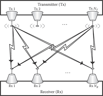Furthermore, stacking together into the vector r_j the KQ consecutive samples collected at the output of the jth receive antenna: rj=[rj(0) rj(Ts) … rj((KQ−1)Ts)]T $r_{j} = {[r_{j} (0) r_{j} (T_{s}) \dots r_{j} ((K Q - 1) T_{s})]}^{T}$ , from Equation 11.39 it follows that:

Images

FIGURE 11.14 An N_T × N_R MIMO system.

r j = α P τ o D H T j, : + n j (11.40)

$r_{j} = α P_{τ_{o}} D H_{j, :}^{T} + n_{j} (11.40)$

where α=Es/NTT−−−−−−−√ $α = \sqrt{E_{s} / N_{T} T}$ , H_j,: denotes the jth column of H, and

P τ = [p - K p (τ) p - K p + 1 (τ) \dots p K + K p - 1 (τ)] P i (τ) = [p (- i T - τ T) p (T s - i T - τ T) \dots p ((K Q - 1) T s - i T - τ T)] T D = [d 1 d 2 \dots d N T] d i = [d i (- K p) d i (- K p + 1) \dots d i (K + K p - 1)] T n j = [n j (0) n j (T s) \dots n j ((K Q - 1) T s)] T

$\begin{matrix} P_{τ} = [p_{- K_{p}} (τ) p_{- K_{p} + 1} (τ) \dots p_{K + K_{p} - 1} (τ)] \\ P_{i} (τ) = {[p (- i T - τ T) p (T_{s} - i T - τ T) \dots p ((K Q - 1) T_{s} - i T - τ T)]}^{T} \\ D = [d_{1} d_{2} \dots d_{N_{T}}] \\ d_{i} = {[d_{i} (- K_{p}) d_{i} (- K_{p} + 1) \dots d_{i} (K + K_{p} - 1)]}^{T} \\ n_{j} = {[n_{j} (0) n_{j} (T_{s}) \dots n_{j} ((K Q - 1) T_{s})]}^{T} \end{matrix}$

The variable K_p stands for the number of symbols affected by the intersymbol interference (ISI) generated by one side of pulse p(t), whose support is − K_pT ≤ t ≤ K_pT. Therefore, the observation interval 0 ≤ t ≤ KT contains contributions from the symbols d(− K_p), …, d(0), …, d(K + K_p − 1). Stacking together all the vectors r_j, j = 1, …, N_R, into the column vector r=[rT1 rT2 … rTNR]T $r = {[r_{1}^{T} r_{2}^{T} \dots r_{N_{R}}^{T}]}^{T}$ yields the modeling equation:

r = α (I N R \otimes P τ o) v e c (D H T) + n, (11.41)

$r = α (I_{N_{R}} \otimes P_{τ_{o}}) v e c (D H^{T}) + n, (11.41)$

where n=[nT1 nT2 … nTNR]T $n = {[n_{1}^{T} n_{2}^{T} \dots n_{N_{R}}^{T}]}^{T}$ , notations ⊗ and vec stand for Kronecker product and vectorization of a matrix (i.e., stacking all the matrix columns one on top of another), respectively, and INR $I_{N_{R}}$ denotes the N_R × N_R unit matrix. Equation 11.41 will prove pivotal in the development of the ML estimator of timing delay τ_o. We will derive the ML timing delay estimator under two general frameworks: the DA ML setup which assumes knowledge of training data (pilot symbols, training sequences), and NDA or blind ML setup in which the transmit data symbols are supposed unknown.

11.8.2.1 Data-Aided Symbol Training Recovery

Using formula vec(ABC) = (C^T ⊗ A)vec(B), the contributions of matrix data D and channel matrix H can be separated in Equation 11.41. It turns out that Equation 11.41 can be recast as

r = α (I N R \otimes P τ o D) v e c (H T) + n . (11.42)

$r = α (I_{N_{R}} \otimes P_{τ_{o}} D) v e c (H^{T}) + n . (11.42)$

Because n assumes a Gaussian distribution, the joint ML estimator of unknown timing delay τ_o and propagation channel h = vec(H^T) is obtained by minimizing the reduced negative log-likelihood function:

$L_{D A} (r | τ, h) = {(r - {\bar{P}}_{τ} h)}^{H} (r - {\bar{P}}_{τ} h), (11.43)$

where ${\bar{P}}_{τ} = α (I_{N_{R}} \otimes P_{τ} D)$ , and τ, h denote trial values for τ_o and vec(H^T), respectively. Equating to zero the gradient of L(r| τ, h) with respect to h, it follows that the ML estimate of channel vector $h ̂$ can be expressed in terms of unknown timing delay as follows:

$̂ h = {({\bar{P}}_{τ} {\bar{P}}_{τ})}^{- 1} {\bar{P}}_{τ} r . (11.44)$

Plugging Equation 11.49 into Equation 11.48 and simplifying, it follows that the ML timing delay estimate must minimize the function:

$L_{D A} (τ) = r^{H} {\bar{P}}_{τ} {({\bar{P}}_{τ} {\bar{P}}_{τ})}^{- 1} {\bar{P}}_{τ} r, (11.45)$

which can be further expanded as

$L_{D A} (τ) = \sum_{j = 1}^{N_{R}} r_{j}^{H} P_{τ} D {(D^{H} P_{τ} P_{τ} D)}^{- 1} D^{H} P_{τ} r_{j}^{H} . (11.46)$

Therefore, the DA ML timing delay estimator can be expressed as

$̂ τ_{M L} = \arg \max_{τ} L_{D A} (τ), (11.47)$

with L_DA (τ) expressed in Equation 11.46 as a sum of N_R terms that depend nonlinearly with respect to τ. Therefore, finding $̂ τ_{M L}$ requires solving a nonlinear optimization problem and no closed-form expression for DA ML estimator is possible. Determination of the global maximum of Equation 11.47 could be performed via a two-step approach. First, a grid-based search might be performed to localize approximately the location of global maxim, which might then be followed by a gradient descent or interpolation-based approach to refine the location of global maximum.

Assuming that the training sequences sent by different Tx antennas are orthonormal, p(t) is a square-root raised cosine pulse and the observation interval K is sufficiently large, then the DA reduced log-likelihood function (11.46) simplifies further to [41]

$L_{D A} (τ) = \sum_{j = 1}^{N_{R}} \sum_{i = 1}^{N_{T}} {| d_{i}^{H} P_{τ} r_{j} |}^{2}, (11.48)$

where $P_{τ} r_{j}$ represents the matched filtering output of the jth Rx antenna with one sample per symbol. Equations 11.46 and 11.48 show that the reduced log-likelihood function for timing recovery in a MIMO system reduces to a sum of N_R reduced log-likelihood functions corresponding to the N_R Rx antennas. This suggests that the tracking and timing estimation techniques from SISO systems could be extended mutatis-mutandis to the MIMO setup.

The performance of the resulting ML timing estimator can be assessed by comparing its mean-square-error (MSE) with performance bounds such as the conditional Cramer–Rao bound (CCRB) [42] and modified Cramer–Rao bound (MCRB) [43]. CCRB represents the Cramer–Rao bound derived under the assumption that the nuisance parameters are treated as deterministic and estimated jointly with the unknown time delay. Proposed as a computational efficient alternative to CCRB, MCRB represents a lower bound to any unbiased estimator, in which the unwanted parameters are averaged out from the log-likelihood function. For a given delay τ_o, CCRB assumes the expression [42]:

$CCRB (τ_{o}) = \frac{N_{o} Q}{2 T t r ({\bar{B}}_{τ_{o}}^{H} S_{\bar{P}}^{⊥} {\bar{B}}_{τ_{o}} C_{h})}, (11.49)$

where tr(·) denotes the trace operator, $B_{τ} = d P_{τ} / d τ, {\bar{B}}_{τ} = d {\bar{P}}_{τ} / d τ, S_{\bar{P}}^{⊥}$ represents the orthogonal projector onto the null space of ${\bar{P}}_{τ_{o}}$ and $C_{h} = Ε (h h^{H}) = I_{}$ . Similarly, the MCRB for a given time delay τ_o can be expressed as [21]:

$MCRB (τ_{o}) = \frac{N_{o} Q}{2 T t r ({\bar{B}}_{τ_{o}}^{H} {\bar{B}}_{τ_{o}} C_{h})} . (11.50)$

Numerical evaluation of Equations 11.49 and 11.50 show that CCRB(τ_o) and MCRB(τ_o) depend inversely proportional with respect to the number of Rx antennas (N_R) [44]. Therefore, the spatial diversity manifests not only through the averaging of N_R SISO log-likelihood functions as in Equation 11.46 but also through the inverse proportional dependence on N_R in CCRB and MCRB. Thus, every increase in the number of Rx antennas (N_R) translates through a proportional reduction in CCRB and MCRB, and, as the computer simulations illustrate in Figures 11.15 and 11.16, in a proportional reduction of the MSE of DA ML estimator. Assuming orthonormal training sequences sent by Tx antennas, Figures 11.15 and 11.16 depict the MSE performance of ML estimator and CCRB for different numbers of Tx and Rx antennas. It turns out that the MSE of DA ML estimator improves when the number of Rx antennas increases, and remains invariant to changes in the number of Tx antennas. The MSE simulation plots also illustrate that DA ML estimator is efficient because it approaches the CCRB. Although not plotted explicitly, numerical evaluations show that in the DA-estimation setup MCRB coincides with CCRB. For the DA synchronization setup, the simulation results shown in Figures 11.15 and 11.16 assumed that the length of training data was 40 (K = 32, K_g = 4), oversampling factor Q = 2, and a square-root raised cosine pulse with roll-off factor 0.3. The timing delay τ_o was uniformly distributed in the interval [0,1), and 10⁴ Monte-Carlo simulations were conducted for each value of τ_o.

Images

FIGURE 11.15 MSE performance of DA ML estimator versus CCRB for different number of Tx antennas.

Images

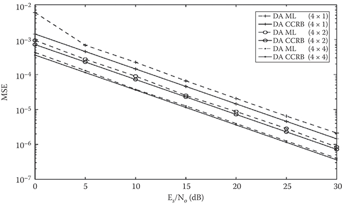
FIGURE 11.16 MSE performances of DA ML and CCRB for different number of Rx antennas.

11.8.2.2 Non-Data-Aided Symbol Timing Recovery

Determination of non-data-aided (NDA) or blind ML estimator for timing delay follows similar steps to the derivation of DA ML estimator. Examining Equation 11.41, it follows that the unknown data matrix D and channel matrix H could be merged together into the unknown vector z = vec(DH^T), and therefore, NDA ML joint estimation of τ and z reduces to the minimization of function:

$L_{N D A} (r | τ, z) = {(r - {\overset{⌣}{P}}_{τ} z)}^{H} (r - {\overset{⌣}{P}}_{τ} z), (11.51)$

where ${\overset{⌣}{P}}_{τ} = α (I_{N_{R}} \otimes P_{τ})$ . Equating to zero the gradient of Equation 11.51 with respect to z, it follows that the ML of z is given by

$̂ z = {({\overset{⌣}{P}}_{τ}^{H} {\overset{⌣}{P}}_{τ})}^{- 1} {\overset{⌣}{P}}_{τ}^{H} r . (11.52)$

Finally, plugging Equation 11.52 back into Equation 11.51, it follows that the NDA ML estimate of τ can be expressed as the argument that maximizes the reduced log-likelihood function:

$L_{N D A} (τ) = r^{H} {\overset{⌣}{P}}_{τ} {({\overset{⌣}{P}}_{τ}^{H} {\overset{⌣}{P}}_{τ})}^{- 1} {\overset{⌣}{P}}_{τ}^{H} r, (11.53)$

which can be further reduced to

$L_{N D A} (τ) = \sum_{j = 1}^{N_{R}} r_{j}^{H} P_{τ} {(P_{τ}^{H} P_{τ})}^{- 1} P_{τ}^{H} r . (11.54)$

Hence, the MIMO log-likelihood function in Equation 11.54 is expressed as a sum of N_R SISO log-likelihood functions corresponding to each of the N_R Rx antennas. As in the DA ML estimation case, in the NDA ML estimation framework, spatial diversity manifests through the exploitation of information (averaging of the log-likelihood functions) at all N_R receive antennas. This remark is enforced by the computer simulations, which illustrate that the MSE performance of NDA ML estimator is inversely proportional to the number of Rx antennas (N_R). Also, the CCRB and MCRB are inversely proportional with respect to the number of Rx antennas. Following the calculations in [42,43], the following closed-form expressions for CCRB and MCRB were found [44]:

$CCRB (τ_{o}) = \frac{N_{o} Q}{2 T t r ({\overset{⌣}{B}}_{τ_{o}}^{H} S_{\overset{⌣}{P}}^{⊥} {\overset{⌣}{B}}_{τ_{o}} C_{z})}, (11.55)$

$MCRB (τ_{o}) = \frac{N_{o} Q}{2 T t r ({\overset{⌣}{B}}_{τ_{o}}^{H} {\overset{⌣}{B}}_{τ_{o}} C_{z})}, (11.56)$

where ${\overset{⌣}{B}}_{τ} = d {\overset{⌣}{P}}_{τ_{o}} /d τ$ , $S_{\overset{⌣}{P}}^{⊥}$ represents the orthogonal projection onto nullspace of ${\overset{⌣}{P}}_{τ_{o}}$ and C_z = E(zz^H).

Assuming the same simulation conditions as in the previous subsection, and QPSK data symbols, Figures 11.17 and 11.18 illustrate the MSE performance of the NDA ML estimator and the corresponding CCRB for different number of Tx and Rx antennas. Similar to the DA ML estimator, the MSE performance of NDA ML estimator is inversely proportional with respect to the number (N_R) of Rx antennas. In addition, the performance of NDA ML estimator is well predicted by the NDA CCRB.

Finally, in Figure 11.19, we plotted the MSE performances of DA ML and NDA ML estimators and their corresponding CCRBs and MCRBs for a 4 × 4 MIMO system. Figure 11.19 shows the superior performance of DA ML estimator relative to NDA ML estimator. This is a reasonable fact because DA ML exploits the additional information given by knowledge of Tx data symbols. Furthermore, Figure 11.19 shows that in the NDA estimation framework, there a significant gap between CCRB and MCRB, a fact which might suggest the existence of NDA estimators with improved performance with respect to NDA ML estimator.

Images

FIGURE 11.17 MSE performance of NDA ML estimator and CCRB for different number of Tx antennas.

Images

FIGURE 11.18 MSE performance of NDA ML estimator and CCRB for different number of Rx antennas.

Images

FIGURE 11.19 MSE performance of DA ML and NDA ML estimators and their CCRBs and MCRBs.

11.8.3 Carrier Recovery in MIMO Systems

Herein subsection, we will consider the carrier synchronization problem in an N_T × N_R MIMO flat-fading channel, where all the Tx/Rx antenna pairs are subject to the same frequency offset F. Assuming perfect timing synchronization (no timing delay τ_o =0), based on Equation 11.39 the output of the jth Rx antenna is modeled as

$r_{j} (t) = \sqrt{\frac{E_{s}}{N_{T} T}} e^{j 2 π F t} \sum_{i = 1}^{N_{T}} h_{i j} \sum_{k} d_{i} (k) p (t - k T) + n_{j} (t) . (11.57)$

Sampling r_j(t) at the symbol period T leads to the discrete-time model for the output of the jth antenna:

$r_{j} (k) = \sqrt{\frac{E_{s}}{N_{T} T}} e^{j 2 π F T k} \sum_{i = 1}^{N_{T}} h_{i j} d_{i} (k) + n_{j} (k), k = 0, \dots, K - 1, (11.58)$

where r_j(k) = r_j(kT) and n_j(k) = n_j(kT). Introducing the vectors: $r (k) = {[r_{1} (k) \dots r_{N_{R}} (k)]}^{T}$ , $d (k) = {[d_{1} (k) \dots d_{N_{T}} (k)]}^{T}, and n (k) = {[n_{1} (k) \dots n_{N_{R}} (k)]}^{T},$ Equation 11.58 is expressed in the equivalent vector-form equation:

$r (k) = α H^{T} d (k) e^{j 2 π F T k} + n (k), k = 0, \dots, K - 1. (11.59)$

Based on Equation 11.59, the DA ML estimates of carrier frequency offset F and unknown channel matrix H are obtained by following the same steps as in the SISO case, and it reduces to the minimization of the nonlinear least-squares criterion:

$L (r | H, F) = \sum_{k = 0}^{K - 1} {| r (k) - α H^{T} d (k) e^{j 2 π F T k} |}^{2} . (11.60)$

Equating to zero the gradient of L(r|H,F) with respect to H and F, it follows that the DA ML estimates of H and F are given by [45]:

$̂ F = \underset{F}{\arg \max} Re [\sum_{k = 0}^{K - 1} R (k) e^{- j 2 π \hat{F} T k}], (11.61)$

$̂ H^{T} = \frac{1}{α} (\sum_{k = 0}^{K - 1} r (k) d^{H} (k) e^{- j 2 π \hat{F} T k}) {(\sum_{k = 0}^{K - 1} d (k) d^{H} (k))}^{- 1}, (11.62)$

where

$R (k) = \sum_{j = k}^{K - 1} r^{H} (j - k) r (j) D (j, j - k)$ and

$D (i, j) = d^{H} (i) {(\sum_{k = 0}^{K - 1} d_{k} d_{k}^{H})}^{- 1} d (j) .$

Similar to the SISO setup, no closed-form expression exists for the DA ML estimator of carrier frequency offset in the MIMO setup. Because finding the maximum of Equation 11.61 is computationally expensive, in practice, sub-optimal but more computationally efficient carrier frequency offset estimators are preferred. An example of such sub-optimal but computationally efficient carrier offset estimator was recently proposed in Reference 45 by mimicking the frequency estimators proposed for SISO channels in [17,18], which basically resumes to weighting appropriately the phases of correlation terms R(k) and taking advantage of diversity offered by the N_R receive antennas. In closing this subsection, we remark that the ML estimator (11.61) is efficient in the sense that it achieves the CRB at medium and high SNRs [45,46].

11.8.4 Conclusions

The slightly more general problem of DA ML joint estimation of carrier frequency offsets and channel gains in a MIMO flat-fading channel with different frequency offsets between different Tx/Rx antenna pairs was recently addressed in Reference 46. However, the more general problem of designing computationally efficient ML algorithms for joint estimation of carrier frequency offsets, timing delays and propagation channel in a MIMO flat or frequency-selective fading channel is still open. Partial attempts based on the use of EM-algorithm and message passing algorithms in factor graphs were proposed for SISO and MIMO joint carrier synchronization and data demodulation. However, the high computational complexity and lack of guaranteed convergence results still prohibit the wide spread of these algorithms to practical systems. Another open research problem is the design of optimal training sequences to reduce the implementation complexity of channel estimation and synchronization algorithms and in the same time to improve the estimation accuracy of channel and synchronization parameters. In this context, [46] developed a set of optimal training sequences that minimize the asymptotic Cramer–Rao bound of carrier frequency offsets in a MIMO system and that also reduce the implementation complexity of the ML estimator.

Good functioning of communication receivers requires proper time and carrier frequency and phase synchronization. Despite the huge advances reported during the last few decades, synchronization continues to represent a complex, and very challenging and important task in the design of any communication system. Furthermore, current developments in the field of telecommunications suggest that more complex and diverse communications systems are being built. Therefore, one expects a proportional increase in the complexity and diversity of the synchronization schemes that will have to satisfy the design challenges and requirements of these new communications systems. It is interesting to observe that current research directions in the field of cooperative (virtual MIMO) wireless communications networks and wireless ad-hoc (sensor) networks bring new challenges in terms of synchronizing the nodes of these networks. These trends have also been visible during the recent years due to the huge interest toward developing efficient synchronization schemes for multicarrier OFDM, OFDMA and MIMO–OFDM systems, as well as for ultra-wideband communication systems.

References

1. J.J. Stiffler, Theory of Synchronous Communications, Englewood Cliffs, NJ, Prentice-Hall, 1971.

2. W. Lindsey and M. Simon, Telecommunication Systems Engineering, Englewood Cliffs, NJ, Prentice-Hall, 1973.

3. H. Meyr and G. Ascheid, Synchronization in Digital Communications, New York, Wiley, 1990.

4. H. Meyr, M., Moeneclaey, and S.A. Fechtel, Digital Communication Receivers, New York, Wiley, 1998.

5. U. Mengali and A.N. D'Andrea, Synchronization Techniques for Digital Receivers, Plenum Press, New York, 1997.

6. F.M. Gardner, Frequency detectors for digital demodulators via maximum-likelihood derivation, Final Report: Part II, ESTEC Contract No. 8022/88/NL/DG, ESA, June 4, 1990.

7. A.N. D'Andrea and U. Mengali, Noise performance of two frequency-error detectors derived from maximum likelihood estimation methods, IEEE Transactions on Communications, 42, 793–802, 1994.

8. A.N. D'Andrea and U. Mengali, Design of quadricorrelators for automatic frequency control systems, IEEE Transactions on Communications, 41, 988–997, 1993.

9. A.N. D'Andrea and U. Mengali, Performance of a quadricorrelator driven by modulated signals, IEEE Transactions on Communications, 38, 1952–1957, 1990.

10. F.M. Gardner, Demodulator reference recovery techniques suited for digital implementation, European Space Agency, Final Report, ESTEC Contract No. 6847/86/NL/DG, August 1988.

11. F.M. Gardner, Properties of frequency difference detectors, IEEE Transactions on Communications, 33, 131–138, 1985.

12. T. Alberty and V. Hespelt, A new pattern jitter free frequency error detector, IEEE Transactions on Communications, 37, 159–163, 1989.

13. M. Moeneclaey, Overview of digital algorithms for carrier frequency synchronization, International ESA Workshop on DSP Techniques Applied to Space Communications, pp. 1.1–1.7, London, UK, September 26–28, 1994.

14. F. Classen and H. Meyr, Two frequency estimation schemes operating independently of timing information, Globecom ’93 Conference, pp. 1996–2000, Houston, TX, USA, November 29–December 2, 1993.

15. F. Classen, H. Meyr, and P. Sehier, Maximum likelihood open loop carrier synchronizer for digital radio, ICC ’93, pp. 493–497, Geneva, Switzerland, 1993.

16. M.P. Fitz, Planar filtered techniques for burst mode carrier synchronization, Globecom ’91, paper 12.1, Phoenix, AZ, December 1991.

17. M.P. Fitz, Further results in the fast estimation of a single frequency, IEEE Transactions on Communications, 42, 862–864, 1994.

18. M. Luise and R. Reggiannini, Carrier frequency recovery in all-digital modems for burst-Mode transmissions, IEEE Transactions on Communications, 43, 1169–1178, 1995.

19. J.C.-I. Chuang and N.R. Sollenbeger, Burst coherent demodulation with combined symbol timing, frequency offset estimation, and diversity selection, IEEE Transactions on Communications, 39, 1157–1164, 1991.

20. Y. Wang, E., Serpedin, and P. Ciblat, Optimal blind carrier recovery for burst M-PSK transmissions, IEEE Transactions on Communications, 51(9), 1571–1581, 2003.

21. Y. Wang, E. Serpedin and P. Ciblat, Optimal blind nonlinear least-squares carrier phase and frequency offset estimation for general QAM modulations, IEEE Transactions on Wireless Communications, 2(5), 1040–1054, 2003.

22. E. Serpedin, G.B. Giannakis, A. Chevreuil, and P. Loubaton, Blind joint estimation of carrier frequency offset and channel using non-redundant periodic modulation precoders, The 9th IEEE Statistical Signal and Array Processing Workshop, pp. 288–291, Portland, OR, Sept. 1998.

23. P. Ciblat, P. Loubaton, E. Serpedin, and G.B. Giannakis, Performance analysis of blind carrier frequency offset estimators for noncircular transmissions through frequency-selective channels, IEEE Transactions on Signal Processing, 50(1), 130–140, 2002.

24. F. Gini and G.B. Giannakis, Frequency offset and symbol timing recovery in flat fading channels: A cyclostationary approach, IEEE Transactions on Communications, 46, 400–411, 1998.

25. Y. Wang, E. Serpedin, P. Ciblat, and P. Loubaton, Performance analysis of a class of non-data aided carrier frequency offset and symbol timing delay estimators for flat-fading channels, IEEE Transactions on Signal Processing, 50(9), 2295–2305, 2002.

26. H.L. Van Trees, Detection, Estimation, and Modulation Theory, New York, Wiley 1968.

27. A. Viterbi, Principles of Coherent Communication, New York, McGraw-Hill, 1966.

28. M. Moeneclaey and G. de Jonghe, ML-Oriented NDA carrier synchronization for general rotationally symmetric signal constellations, IEEE Transactions on Communications, 42, 2531–2533, 1994.

29. C.N. Georghiades, Blind carrier phase acquisition for QAM constellations, IEEE Transactions on Communications, 45, 1477–1486, 1997.

30. M. Morelli, A.N. D'Andrea, and U. Mengali, Feedforward estimation techniques for carrier recovery in 16-QAM modulation, in M. Luise and S. Pupolin (Eds.) Broadband Wireless Communications, Springer-Verlag, London, 1998.

31. E. Serpedin, P. Ciblat, G.B. Giannakis, and P. Ciblat, Performance analysis of blind carrier phase estimators for general QAM constellations, IEEE Transactions on Signal Processing, 49(8), 1816–1823, 2001.

32. F. M. Gardner, Phaselock Techniques, 3rd edition, 2005, John Wiley & Sons.

33. K.H. Mueller and M. Muller, Timing recovery in digital synchronous data receivers, IEEE Transactions on Communications, COM-24, 516–531, 1976.

34. O. Agazzi, C.-P.J. Tzeng, D.G. Messerschmitt, and D.A. Hodges, Timing recovery in digital subscriber loops, IEEE Transactions on Communications, COM-33, 558–569, 1985.

35. F.M. Gardner, A BPSK/QPSK Timing-error detector for sampled receivers, IEEE Transactions on Communication, COM-34, 423–429, 1986.

36. C.N. Georghiades and M. Moeneclaey, Sequence estimation and synchronization from nonsynchronized samples, IEEE Transactions on Information Theory, 37, 1649–1657, 1991.

37. J.L. Massey, Optimum frame synchronization, IEEE Transactions on Communications, COM-20, 115–119, 1972.

38. R.H. Barker, Group synchronization of binary systems, Communication Theory, W. Jackson Editor, London, pp. 273–287, 1953.

39. F. Neuman and L. Hofman, New pulse sequences with desirable correlation properties, Proceedings of the National Telemetry Conference, Washington, DC, pp. 272–282, 1971.

40. P.T. Nielsen, On the expected duration of a search for a fixed pattern in random data, IEEE Transactions on Information Theory, September, 702–704, 1973.

41. Y.C. Wu, S.C. Chan and E. Serpedin, Symbol-timing estimation in space–time coding systems based on orthogonal training sequences, IEEE Transactions on Wireless Communications, 4(2), pp. 603–613, 2005.

42. J. Riba, J. Sala, and G. Vazguez, Conditional maximum likelihood timing recovery: Estimators and bounds, IEEE Transactions on Signal Processing, 49, 835–850, 2001.

43. A.N. D'Andrea, V. Mengali, and R. Reggiannini, The modified Cramer–Rao bound and its application to synchronization problem, IEEE Transactions on Communications, 42, 1391–1399, 1994.

44. Y.C. Wu and E. Serpedin, Symbol timing estimation in MIMO correlated fading channels, Wireless Communications and Mobile Computing (WCMC) Journal, Wiley, 4(7), 773–790, 2004.

45. F. Simoens and M. Moeneclaey, Reduced-complexity data-aided and code-aided frequency offset estimation for flat-fading MIMO channels, IEEE Transactions on Wireless Communications, 5(6), 1558–1567, 2006.

46. O. Besson and P. Stoica, On parameter estimation of MIMO flat-fading channels with frequency offsets, IEEE Transactions on Signal Processing, 51(3), 602–613, 2003.

Table of Contents for
11 Synchronization of Communication Receivers

11

Synchronization of Communication Receivers

11.1 Introduction

11.2 Carrier Synchronization

11.2.1 Carrier Frequency Synchronization

11.3 Carrier Phase Synchronization

11.3.1 Unmodulated Carrier

11.3.2 Synchronization from a Modulated Carrier

11.4 Carrier Acquisition for QAM Constellations

11.5 Symbol Synchronization

11.6 To Browse Further

11.7 Frame Synchronization

11.7.1 Performance

11.8 Synchronization of MIMO Systems

11.8.1 General Considerations

11.8.2 Timing Recovery in MIMO Systems

11.8.2.1 Data-Aided Symbol Training Recovery

11.8.2.2 Non-Data-Aided Symbol Timing Recovery

11.8.3 Carrier Recovery in MIMO Systems

11.8.4 Conclusions

References

Further Reading

Table of Contents for 11 Synchronization of Communication Receivers

Create new playlist

Sign In

Sign Up

11

11.8.2.1 Data-Aided Symbol Training Recovery

11.8.2.2 Non-Data-Aided Symbol Timing Recovery

Table of Contents for
11 Synchronization of Communication Receivers