Chapter 3. Creating the data mart

This chapter is recommended for

	Business analysts
	Data architects
	Enterprise architects
	Application developers

Mondrian makes it easy for users to do analysis, but behind the scenes it requires data organized in a way that’s convenient for analysis. Historically data has been organized for operational use in third normal form (3NF), but Mondrian has adopted the use of star schema structures based on industry best practices.

In this chapter, we’ll cover the general architecture of an analytic solution and then explore star schemas, the “best practice” database modeling technique for analytic systems. We’ll dig into their specifics, understanding that Mondrian is expecting to perform its analytic magic on top of a star schema. We’ll compare this with third normal form modeling and examine some of the high-level benefits of the star schema for an analytic system.

We’ll conclude with a few additional aspects of the star schema technique, including how to manage changes to data over time, modeling the all-important time dimensions.

By the end of this chapter, you’ll understand how data is structured to make analysis with Mondrian possible. This chapter is primarily aimed at the data architect, but other readers will likely find understanding the data architecture useful as well.

3.1. Structuring data for analytics

Before we can get into the details of how to build the underlying physical architecture, it’s helpful to understand what we’re trying to accomplish and the high-level architecture required to meet these goals. In this section, you’ll learn why a particular database architecture is needed and how it aids in analysis. By the end of the section, you should understand what a star schema is and how it supports the goals of online analytic processing.

3.1.1. Characteristics of analytic systems

As the data warehouse (DW) or business intelligence (BI) architect or developer for Adventure Works, you’re charged with making sure the analytics presented to your users exhibit the following three characteristics:

• Fast —Users expect results at the “speed of thought,” and the fact that your database is scanning millions of transactions to build these results is irrelevant to them. If you haven’t presented them with the results quickly enough for them to continue asking questions, refining their results, and exploring, you’ve lost them.

  Fast Rule of Thumb

  If the reporting results take long enough that the user considers going to refill their coffee, your solution isn’t fast enough.

• Consistent and accurate —Nothing drives users more insane than running two reports in a system and getting results that don’t match. For instance, if your OLAP system produces reports on sales by quarter and by year, and the quarterly totals don’t add up to the yearly total (as in table 3.1), your users will lose confidence in how accurate the analytics presented by your system are. Your solution must never present results like these.

  Table 3.1. Inconsistent and inaccurate results are bad

  Year	Quarter	USD sales
  2012	Quarter 1	$50
  2012	Quarter 2	$50
  2012	Quarter 3	$100
  2012	Quarter 4	$100
  2012	All Quarters	$350—Different!

• Information focused —Users don’t care that the SKU for the product is contained in the column UNIQUE_RESOURCE_LOCATOR in their ERP source system and that it’s in the PLU_BASE_UNIT column in the CRM tool. The analytics you present in your OLAP system must focus on the information subjects, such as sales and customers, that are analytically significant to your users. Users want to see the customer name “Bob” and the state “California” instead of the transactional IDs for the values (100, 22CA1, and so on). ERP and CRM systems use IDs and codes, but users think in names and labels. Additionally, transactional (OLTP) systems, like your CRM and ERP, change over time. The OLAP system needs to handle data changes with grace, and delivering reports in terms of information subjects insulates you somewhat from these inevitable changes. Your company may someday move from Oracle Applications to Salesforce.com, but if your analytic system is just sales and customers, this change need not affect the reports.

If you’ve worked with technology for any period of time, you’re likely thinking that the fast, consistent, and information-focused objectives aren’t implemented easily. These objectives are not the low-hanging fruit that the installation of a single piece of software can achieve. Let’s look at the architectures that will help you achieve these characteristics.

3.1.2. Data architecture for analytics

Fortunately for all of us, building analytic systems to meet the objectives outlined in the previous section is not new. Many thousands of professionals—numerous authors, experts in the industry, and vendors—have spent years refining the tools, techniques, and best practices for implementing analytic systems that are fast, consistent, and information focused.

This collective wisdom boils down to two almost universally accepted tenets of building analytic systems:

• Copy data to systems dedicated for analytics —Data, unlike physical assets, can be duplicated with relative ease. Your transaction systems require advanced security and high availability, and they’re designed to be fully available to run your company. They are, generally speaking, ill-suited to performing aggregations across many areas, such as multitable joins, and typically include analytic reporting as a bolt-on piece of the primary application. Doing analytics on these systems is a common source of poor system availability and high system loads. If you’re reading this, there’s a decent chance that you’ve received an email from a DBA or system administrator complaining about a running query that’s slowing down the whole system.
• Transform, clean, and enrich data for analytics —While these transactional systems tend to be flexible, they speak a foreign language of codes, effective dates, keys, composite keys, and joins. Data is what transactional systems are built to manage, but that’s not what matters to the analytic users. The industry knows that in order for the data to be useful, it must undergo a transformation from data (in the form of CSV files or raw tables in a database) into information subjects such as sales or customers. Often, the data necessary to do an analysis isn’t even present in the original data stream, and integrating, matching, and enriching this data in the analytic system is necessary to present certain analytics. The act of moving data from the source system to the analytics system is referred to as extract, transform, and load (ETL).

Whether you’re working with a data warehouse that serves as the long-term storage of company data, a single analysis area commonly called a data mart, or an interdependent set of data marts, the industry has determined that analytics should be done on separate computer resources and include data that has been cleaned, transformed, and enriched from multiple source systems. Figure 3.1 shows an overview of a typical analytic environment with separate source systems and analytic systems. Data is copied to the analytic environment via ETL, and users access their reports and data in the analytic environment rather than working directly against the source systems.

Figure 3.1. Analytic architecture overview: data is copied (and enriched) from the source systems to a dedicated analytic environment, which is where users (via Mondrian) access analytic data.

3.1.3. Star schemas

The common need for analytic systems that are fast, consistent, and information focused has led the industry to a widely accepted best practice of dimensional modeling based on the physical star schema methods. We’ll briefly explain the basics of the star schema and how it meets these goals, and compare it with third normal form modeling (3NF).

The star schema is an industry best-practice modeling technique optimized for massive, dynamic aggregations. 3NF modeling is the industry best practice for modeling transactional systems (OLTP), but star schemas are the best practice for analytics (OLAP). The concepts and specifics are outlined comprehensively in the authoritative book on the topic by Ralph Kimball and his colleagues, The Data Warehouse Lifecycle Toolkit, 2nd edition (Wiley, 2008). If you’re looking for more advanced techniques or greater detail on any concepts introduced and intentionally kept brief in this chapter, we encourage you to refer to that book. We’ll cover, later in this chapter, some of the reasons a star schema is a best practice and its numerous benefits.

For all intents and purposes, Mondrian expects your data to be in a relational database, in the star schema format (or one of its closely related permutations). The star schema, as a set of relational database tables, is what Mondrian uses as the basis to perform aggregations and analytics.

We’re going to cover the general structure of a star schema, but it’s worth noting that the specifics of each individual business model are driven by the analysis needs of that particular company, department, or user. In chapter 2, we noted that the desired analytics and model for Mondrian cubes drive the design of both the Mondrian schema and the star schema that supports it. To understand how the analytic needs of users drive the actual implementation model, we’ll use Adventure Works as an example.

Adventure Works managers want to understand how much revenue they’re selling to which types of customers. They’re looking to understand, first, their sales by customer state. They’ll eventually wish to look at additional attributes, such as sales over time, but for our first foray into star schemas, the basic request for sales by customer state will suffice.

Mondrian and star schemas

Mondrian expects your data to be in a relational database, in a star schema which is an industry best-practice modeling technique for OLAP systems.

A star schema consists of a fact table surrounded by multiple dimension tables. The shape of a fact surrounded by dimensions is how the star schema gets its name.

Fact tables contain the stuff you’re trying to aggregate, total, and measure. The numbers that are added together to create the total sales number are contained in the fact table and are referred to as the measures in the cubes (more on this in chapter 4). The measures are the what you’re trying to measure and analyze. In our example and figure 3.2, sales is the what we’re trying to measure.

Figure 3.2. Star schema. The fact contains the what you’re trying to measure—sales, and more specifically the column that has the data to be aggregated, sales_amount. The dimensions are the by attributes that you’re trying to segment and allocate the data to—customer, and more specifically the state the customer is from, customer_state.

Dimension tables contain the qualifying attributes that you want to split out those numbers (the measures) by. In our example and figure 3.2, the users wish to split out the total sales (in the fact table) by customer state, so that you can see the total sales for each state individually, along with the total sales for all states. Customer state is the by that you are trying to use for comparison and filtering.

What you are trying to measure (revenue, web impressions, customer calls, and so on) is in the fact table. The things you are trying to split it out by (product, geography, and the like) are in the dimension tables.

When looking at the physical database model, a star schema consists of the following:

• Dimension tables that contain rows, independent of the transactions that have the attributes. For instance, a product dimension would contain a row per product and contain information on product categories, vendors, departments, and the like. Typically this foreign key is also non-nullable, so that you can aggregate the table at any combination of dimensions and always get the same sum total. Remember, consistency is one of the goals, and this ability to aggregate at any combination of dimensions helps keep the sum totals consistent, avoiding the results in table 3.1.

  Simple example without history

  This design, with a single row per product, is a simple example for a Type I dimension. Please see section 3.2.1 on Slowly Changing Dimensions later in this chapter for more detailed discussion of keeping history for dimensions.

  Dimension tables are highly denormalized with many columns when compared to their original source system tables. Your source system may have included information about departments in a table separate from employees, but in the star schema the department name is now a column in the employee dimension.
• A single fact table that contains a row for the individual transactions (order line items, individual clicks) matching the grain of the table (see Kimball’s book for more information on “grain”). The fact table contains a set of surrogate integer keys that easily join to the dimension tables for the attributes associated. Additionally, it will usually have one or more columns that contain the values to be aggregated, associated with that single transaction.

The other thing to note is that using this technique means that fact tables typically contain at least 10 times, but more commonly at least 1000 times, more records than the dimension tables. Fact tables contain millions to billions of rows, and dimension tables typically contain thousands to just a few million. This has important performance benefits, and it’s a key reason why this modeling technique can deliver speedy results even when millions of facts are involved.

3.1.4. Comparing star schemas with 3NF

Given that you’re reading this book, you’ve likely either designed, built, maintained, or optimized a database schema for an application. We’ll review the technique and then examine why we’ll depart from it and use the star schema.

As a brief refresher, 3NF is a modeling technique in which redundancy is reduced, and foreign keys are introduced so that additional attributes (such as the name of the state) are located in a different location and must be accessed in another table.

The 3NF model has been blessed as the “correct” database modeling technique with little discussion or questioning. 3NF is, for the most part, the best model for transactional systems like an ERP or CRM. The 3NF modeling techniques are ideal in the following situations:

• Lots of concurrent users reading and modifying data —Keeping similar data together, and factoring out and normalizing repetitive data (such as department names, locations, and the like) allows lots of users to operate on smaller sections of the dataset independently and without conflicts (or locks).
• Subprograms and people are accessing small slices of data —Typically users of an HR system are not going to update the last name of every employee in the company. They will, more likely, access a single employee and update the last name of a single record.
• Source systems usually access smaller slices of data joined together with a foreign key —These joins are inexpensive with a relatively small amount of data. Databases, to reassemble a complete order with line items, typically need to do two small indexed reads into two tables (for example, retrieving the orders from one table and line items from another). Reading two different locations is a small amount of overhead when dealing with a single order.

The 3NF technique is not, however, a good model for a few users doing large aggregations touching entire sets of data. Joining a single record to others (a small amount of data) tends to be efficient. Joining many tables, to include all the attributes used for qualification (large numbers of database rows) requires much more work by the database. You’ve likely written a few SQL statements for your reports that are a page or two themselves, and their database EXPLAIN is a small chapter of a book; these queries tend to perform poorly as the dataset grows in size. We certainly wrote our share of these expensive, poorly performing queries before embarking on our OLAP adventures.

If you’re accustomed to 3NF modeling, the first star schemas you design will not feel “right.” They’ll leave you with a strange, lingering feeling that you’ve just built a terrible data model. Over time, though, as the fit between the star schemas and the use cases becomes increasingly apparent, the modeling technique won’t feel quite so strange.

3.1.5. Star schema benefits

We can’t cover all the benefits of the star schema in this book, but at a top level, the star schema has the following benefits:

• Star schemas require at most one pass through the table. There’s no need to look over millions of records time and again; the database will simply make one pass aggregating the dataset. The single remaining join path is centered on the largest table. Database planners typically produce efficient executions when cardinality differences between tables are large. Identifying which tables will be expensive (and drive the single-pass approach) and which tables are smaller lookup tables makes the planner’s job straightforward.
• Missing join keys don’t cause sum-total issues in star schemas. Consider the difficulty in balancing sum totals if some products are not assigned to categories. If you join via a key that isn’t present, and the join condition in SQL isn’t satisfied, you typically lose records before doing the aggregations. In this situation, it’s possible to do an aggregation without a GROUP BY statement and get one figure, and then to get different totals if you join to a table. With a star schema, you can mix and match and do aggregations at the intersection of any attributes and always come up with the same exact sum total of revenue. You can probably think back to a SQL report you’ve written that joins to an extra table for an additional reporting field. All of a sudden, the users’ sum totals are missing due to missing join keys. Star schemas help you avoid this pitfall; you must include a dimension record that serves as the star schema equivalent of NULL so that fact records that don’t have the attribute always join to every dimension.
• Many databases have physical optimizations for star schemas. The star schema eliminates multitable joins, which are extremely inefficient and costly to perform on large sets of data. A single, easy to optimize physical structure (one large table, and single-key joins to surrounding smaller tables) is something that nearly every database can perform effectively. Further, expecting this particular modeling technique and seeing the physical tables organized as a star schema, some databases have features that provide even greater efficiencies and query speed improvements. Bitmap indexes, parallel query and partitioning, and sharded fact tables are just a few of the techniques. In fact, there’s an entire class of column storage databases that are purposely built to handle such schemas/workloads and provide blazing fast performance on top of star schemas.
• Star schemas are the preferred structure for Mondrian, but they’re also easier for anyone writing SQL. Although the primary consumer for a star schema is an OLAP engine like Mondrian, the database and tables themselves represent an information-focused, easy-to-understand view of the data for reporting. A star schema reduces the complexity and knowledge necessary to write plain old SQL reports against the data. Analysts who typically needed to remember complicated join rules (such as remembering to include an effective date in the SQL join so you don’t get too many records and double-count your sales) have a simplified information-focused model to report against.

Now that we’ve looked at the basic structure and benefits of star schema design and compared it to 3NF techniques, it’s time to delve into some further techniques that will almost certainly be required with a star schema of any real complexity.

3.2. Additional star schema modeling techniques

You’ve learned what star schemas are and why they’re useful. In this section, we’ll cover some additional aspects of star schema modeling. These additional techniques and patterns fall into two different categories:

• Techniques for handling changes to dimension data over time —Products change categories, stores change attributes, and so on. You need to be able to handle changes to your dimensions over time using Slowly Changing Dimension techniques.
• Performance enhancements —We’ll cover some techniques for improving the overall performance of the system.

3.2.1. Slowly Changing Dimensions (SCDs)

Slowly Changing Dimensions (SCDs) are dimensions that change slowly over time, and in this section we’ll look at techniques for handling changes to dimensional attributes. The “slowly” need not connote any particular rate of change; data can change frequently throughout a day or change once or twice per year. The key aspect we’ll try to model and solve is how to handle these changes to data and ensure that we properly account for changes over time.

Industry-standard descriptions of SCD techniques have been developed; they aren’t particular to Mondrian but are broadly applicable to star schemas for other OLAP products as well. The three types of SCDs (I, II, and III) were initially outlined in Kimball’s definitive and timeless work on dimensional modeling, The Data Warehouse Lifecycle Toolkit, 2nd edition (Wiley, 2008), and while some additional permutations of these types exist, the three types cover nearly all use cases.

It’s easiest to explain SCDs through an example. We’ll examine a customer named Bob, the sales associated with him, and the changes to his data over time. We’ll look at how we can manage changes to Bob’s data over time.

In the source CRM system, the customer records for Bob are stored in CRM_TABLE (figure 3.3). Bob has a single record in this table, and the table is updated as changes are made (such as by a customer service agent using the CRM software). There is a single, up-to-date version of Bob in the CRM system.

Figure 3.3. Source data in the CRM system. A single record per customer in CRM_TABLE is uniquely identified by CRMID, with sales transactions related to a customer being referenced through a foreign key in CRM_SALES.

Purchases made by Bob are recorded in the same system, in the CRM_SALES table. Bob lived in California (CA) until June 2002, at which point he moved to Washington (WA). This table contains the date of the sales transaction, foreign key references to Bob’s CRM ID (100), and the transaction amount. This is a simplistic (and perhaps a little oversimplified) version of the way data is commonly represented in source systems.

-- Before June 2002
select * from CRM_TABLE;
+-------+------+-------+
| CRMID | NAME | STATE |
+-------+------+-------+
|   100 | Bob  | CA    |
+-------+------+-------+

-- After June 2002
select * from CRM_TABLE;
+-------+------+-------+
| CRMID | NAME | STATE |
+-------+------+-------+
|   100 | Bob  | WA    |
+-------+------+-------+

-- All of Bobs sales
select * from CRM_SALES;
+---------+------------+--------+-------+

| SALESID | SALESDATE  | AMOUNT | CRMID |
+---------+------------+--------+-------+
|    1001 | 2001-01-01 |    500 |   100 |
|    1002 | 2002-02-01 |    275 |   100 |
|    1003 | 2003-09-01 |    999 |   100 |
+---------+------------+--------+-------+

Given your new understanding of star schemas, it’s probably clear at this point that because sales are the what that you’re trying to measure, sales will be a fact table in the star. It would also be common to want to see sales by customer state (the by). Reinforcing what you saw earlier in figure 3.3, you know that the by attributes (customer state) will be in a dimension table. Now we simply need to address the challenge that arises from Bob moving from CA to WA in June 2002.

The challenge, of course, is determining how to appropriate certain sales amounts in Mondrian and the star schema in keeping with the business requirements. In our example, Bob made two purchases (2001-01-01 and 2002-02-01) while he lived in California. The big question, and the one we can address with one of our SCD techniques, is whether those two sales amounts ($500 and $275) should be totaled in California (where Bob lived when he made those purchases) or in Washington (where Bob resides now). The three SCD techniques give us the ability to achieve the results Adventure Works desires.

SCD Type I

SCD Type I is a dimensional modeling technique that, as in our example source system, keeps a single version of the entity. In our example, Bob just has a single record in a customer dimension table (figure 3.4). As Bob changes attributes (from CA to WA), his record is updated in the table; no history of changes is kept. The fact table records have a reference to the dimension record for Bob.

Figure 3.4. Type I dimension tables. Notice that the foreign key from the fact table to the dimension table is the single-source system identifier CRMID. Given that this is the primary key for the dimension table, it’s clear that there’s only one record for Bob in the dimension.

-- Dimension Table (Type I).  No History, single version of Bob
select * from dim_customer_type_I;
+------------+------------+-----------+
| cust_CRMID | cust_state | cust_name |
+------------+------------+-----------+
|        100 | WA         | Bob       |
+------------+------------+-----------+


-- Fact Table (Foreign Key to Customer dimension is cust_CRMID)
select * from fact_sales_type_I;
+---------------+--------------+------------+------------+
| fact_sales_id | sales_amount | sales_date | cust_CRMID |
+---------------+--------------+------------+------------+
|          1001 |          500 | 2001-01-01 |        100 |
|          1002 |          275 | 2002-02-01 |        100 |
|          1003 |          999 | 2003-09-01 |        100 |
+---------------+--------------+------------+------------+

-- Typical Mondrian Star Query (sum measure, group by dimension)
select
  sum(sales_amount) as 'sales',
  cust_state
from
  fact_sales_type_I f,
  dim_customer_type_I d
where
  f.cust_CRMID = d.cust_CRMID
group by
  cust_state;
+-------+------------+
| sales | cust_state |
+-------+------------+
|  1774 | WA         |
+-------+------------+

In the preceding code example, notice the query to the star schema that Mondrian will issue to present the total sales by state view. You’ll notice that since there’s a single record for Bob, and his state is current, indicating that he’s living in WA, all of Bob’s sales are now considered to be WA sales. This is the key attribute of Type I SCD dimensions; changes are made to the single record, and all previous transactions are now included in the new value totals. Even though Bob lived in CA for his first two purchases ($500 and $275), they don’t show up in CA; the entire amount of $1,774 is included in WA.

Type I dimensions are often used for items that don’t change frequently (country names, area codes, and the like), and when they do change, they represent a true update or correction of the data. For instance, if the name of a country changes (“Suessville” to “Democratic Peoples Republic of North Suessville”), it’s unlikely that business users will want to see two different figures (old name and new name) and two different names. For such an update, all records (old transactions and new ones) should be included in the new name.

SCD Type II

SCD Type II dimensions keep a history of changes to the attributes of the dimension. In our example, Bob would have two records in the customer dimension. One record represents the period from when he became a customer in 1980 up until he moved to Washington—in this record his state is CA. The second record covers his time living in Washington. These versioned records of Bob represent him at particular points in time.

For Type II dimensions, a surrogate key is created to uniquely identify a particular version (such as 8888 or 8889) of the natural key (Bob, CRMID 100). For Type II dimensions, the surrogate key is meaningless and it’s used only as a simple, single-key join from the fact table.

There is a new unique key that’s normally omitted from the physical database schema but is a logical constraint: a combination of the natural key (CRMID) and the effective date identifies unique records in a dimension (figure 3.5).

Figure 3.5. Type II dimension tables.

When loading the fact table, the ETL system examines the date of the sale (sales_date) and chooses which version of the dimension key to use. In our example, two of Bob’s transactions use the record where he lived in CA (8888) for a foreign key, and his last transaction uses his current effective record (8889) as a foreign key. It is this versioning, and the ability of the fact table to join to different versions of the same entity, that give SCD Type II dimensions the ability to attribute historical transactions to the correct attributes.

-- Bob now has TWO records in the dimension, and when the new record was
-- effective.  Notice the surrogate key is now the PK for the table
select * from dim_customer_type_II;
+-----------------+---------------+----------------+-------+------+
| dim_customer_id | nat_key_CRMID | effective_date | state | name |
+-----------------+---------------+----------------+-------+------+
|            8888 |           100 | 1980-01-01     | CA    | Bob  |
|            8889 |           100 | 2002-06-01     | WA    | Bob  |
+-----------------+---------------+----------------+-------+------+

-- Now, Bob's sales point to one of his two different dimension versions
-- The two records before June 2002, point to his first record (8888)
-- The record AFTER he moved, point to his second record (8889)
select * from fact_sales_type_II;
+---------------+--------------+------------+-----------------+
| fact_sales_id | sales_amount | sales_date | dim_customer_id |
+---------------+--------------+------------+-----------------+
|          1001 |          500 | 2001-01-01 |            8888 |
|          1002 |          275 | 2002-02-01 |            8888 |
|          1003 |          999 | 2003-09-01 |            8889 |
+---------------+--------------+------------+-----------------+

-- Now, when creating the sales Star query, the results put Bobs
-- sales when he lived in CA into CA, and when he lived in WA
-- into WA.  Notice the query has no date management; this has

-- already been done when choosing which version of Bob from
-- the dimension table (8888 or 8889).
select
  sum(sales_amount) as 'sales',
  cust_state
from
  fact_sales_type_II f,
  dim_customer_type_II d
where
  f.dim_customer_id = d.dim_customer_id
group by
  cust_state;
+-------+------------+
| sales | cust_state |
+-------+------------+
|   775 | CA         |
|   999 | WA         |
+-------+------------+

Notice that the same SQL query to sum sales now returns totals that put Bob’s purchases into the state he was living in when he made the purchase. His $500 and $275 sales in CA are totaled in CA ($775), and his $999 purchase after he moved is attributed to WA.

SCD Type II dimensions are used when a history of changes and attributes is needed. This is very common, and Type II dimensions are used much of the time. You can understand the rationale; business users want accurate per-state sales. They dislike when reports magically move historical data from one line to another; historical data should be settled, finished data.

Type II dimensions often include additional columns for easy management and lookups, even if they aren’t required. It’s common to see an expiration date, in addition to an effective date, so that the SQL that looks up the dimension can use a straightforward BETWEEN clause rather doing a MIN(effective) where date is greater than effective. It’s also not uncommon for a version identifier to be present (1, 2, 3, ...); it’s superfluous, but it makes it easy to numerically identify versions of the entity.

SCD Type III

Type III dimensions are somewhat rare; we’ll cover them briefly, and you can look into online resources or other books to dig into the details and some examples. Our example of Bob’s purchase history doesn’t fit with a classic Type III use case.

Type III dimensions are used when you want to keep both attributes around and be able to use either to classify the results. Type III dimensions are often used when you bring in a second classification system, and you don’t think of it as a “change” so much as an additional method of bucketing or classifying.

Take, for instance, a sales organization that’s reorganizing. Perhaps they were split into four regions before the reorganization (West, Central, East, and International) and they’re moving to another system (North, South, International Europe, International Asia). For a while, given that commissions, sales bonuses, and other key company metrics will need to be determined using the old system while the new system is being rolled out, you’ll need to be able to use both methods. You’ll need to roll up your sales by both the new sales regions and the old sales regions.

This is typically accomplished by adding a column to an existing dimension (Type I or Type II) that retains both sets of regions. In our continuing example, there’d be two columns in the dimension: NEW_REGION would contain the new region names for that salesperson, and OLD_REGION would contain the old region names. This enables a type of dual taxonomy analysis, allowing the user to explore either region.

SCD summary

All three types of dimensions can be used, depending on the particular business needs associated with the dimension. A single star schema can mix and match different types of dimension tables, so choosing a Type I for a particular dimension doesn’t mean that for another dimension for the same fact table you can’t use Type II.

As a general rule, most dimension tables use Type II dimensions, probably followed by Type I. Type III dimensions are rare and represent a small number of use cases. If you’re new to dimensional modeling and your experience doesn’t automatically tell you how to model the dimension you’re adding, start by assuming it’ll be a Type II dimension, and then adjust it only if you see the telltale signs that it’s a Type I or Type III.

Having covered the methods available for addressing business needs for data changing over time, let’s move on to discuss other modeling techniques for performance and enhanced functionality.

3.2.2. Time dimensions

Time dimensions are critically important to OLAP systems; almost every single system has some sort of time component associated with it, and it’s very rare for watching metrics over time to not be a key requirement. It’s almost a foregone conclusion that for whatever system you build using Mondrian, you’ll have some sort of time dimension. Time dimensions are, for the most part, like any other dimension. In fact, with the exception of a single configuration in Mondrian to enable some powerful time-centric MDX shortcuts (such as year-to-date aggregations or current period versus prior period, and the like), time dimensions are exactly like any other dimension table. We’ll look at how you can make Mondrian aware of your time dimension in chapter 4.

Time dimensions are denormalized Type I dimensions where the natural (and usually the primary) key is the date. Type I is almost always appropriate because the attributes rarely change. For instance, July 01 2005 will always be a Friday. Its attributes (the fact it was Friday, was in July, and so on) won’t ever change, so managing changes for time dimensions is usually not necessary.

All of the relevant pieces of the date, such as the month name, quarter, and day of the week, are denormalized and included as columns in the table. If you’ve created SQL reports before, you might be wondering why this is done. After all, extracting the month number from a date is a straightforward function. Usually something like select month(date) from table can quickly and easily extract the information. But there’s a good reason to denormalize it: performing the same calculation, extracting the same exact integer (7 for our July example) from the date (July 01 2005) millions of times with every query, means performing a lot of unnecessary work in the database. Also, some database optimizers can optimize, group by, and filter clauses on straight integer columns (such as MonthNumberOfYear) but have a much harder time optimizing and grouping or filtering on a function, such as month(date). See figure 3.6.

Figure 3.6. Time dimension: all the attributes of a date are denormalized and presented as real textual values. Even though extracting the month number from the date is possible, a denormalized and repetitive column (MonthNumberOfYear) is created for easy and high-performance grouping and filtering for star queries.

+----------+--------------+-----------+------------+---------------+
| DateKey  | CalendarYear | MonthName | FiscalYear | FiscalQuarter |
+----------+--------------+-----------+------------+---------------+
| 20050701 |         2005 | July      |       2006 |             1 |
| 20050702 |         2005 | July      |       2006 |             1 |
| 20050703 |         2005 | July      |       2006 |             1 |
| 20050704 |         2005 | July      |       2006 |             1 |
| 20050705 |         2005 | July      |       2006 |             1 |
| 20050706 |         2005 | July      |       2006 |             1 |
| 20050707 |         2005 | July      |       2006 |             1 |
| 20050708 |         2005 | July      |       2006 |             1 |
| 20050709 |         2005 | July      |       2006 |             1 |
| 20050710 |         2005 | July      |       2006 |             1 |
+----------+--------------+-----------+------------+---------------+

In addition to the performance benefits of having all the regular pieces of the time dimension denormalized, there’s another benefit. It’s very common for organizations to have additional columns and attributes that need to be used for analysis just as frequently as the standard calendar attributes. The most common of these is the fiscal calendar in use by a company, which is typically offset a few months from the Gregorian calendar. Fiscal attributes (such as fiscal year, quarter, and so on) can be added as additional columns to the time dimension.

In some ways, the time dimension is a very effective part of the solution. When a fact table joins to a single date in the time dimension, a wide variety of time-based aggregations involving different categories, calendars, retail schedules, and so on, are all possible without any additional work. In other words, a well-designed time dimension means the fact table designers and ETL developers don’t have to worry about how to roll up these transactions by fiscal and Gregorian calendar attributes.

Notice in figure 3.6 that the primary key for the time dimension is an integer—a coded version of the date. July 01 2005 is the integer 20050701. This is a common trick, so that when loading a fact table you don’t have to do a table lookup to find the time dimension record that matches your date. A little date munging, and you can determine the integer for your desired date, without ever having to ask the database for that information. When you’re loading millions of rows, this is a helpful little optimization.

Notice that the time dimension has only a day portion but does not include any intra-day attributes (such as hour, minute, and so on). Including down to the minute or second values would make the dimension table much bigger and reduce some of the performance benefits of having dimension tables with fewer records joined to fact tables that have large numbers of records. If intra-day analysis is needed, this is commonly addressed by adding a separate time of day dimension that’s separate from the time dimension and that has attributes for the intra-day divisions (hour, minute, and the like).

In section 11.1.3, we’ll cover some of the very powerful MDX extensions available for time dimensions. Once these extensions are configured in Mondrian, common analytic questions (this year to date versus last year to date at the same point) become very easy in MDX. Additionally, most ETL products have some sort of time dimension generator, and there are even websites where you can get fully baked time dimensions (data and database table definitions). PDI includes a time dimension generator in its sample directory, and Mondrian 4 has added the ability to create time dimensions automatically.

3.2.3. Snowflake design

Using a star schema is considered a best practice, and this design should be used for Mondrian in almost all cases. But as usual, there are some use cases where it’s appropriate to break the rules; you can use one level of normalization on dimensions (an additional join) for various operational and performance reasons. In this approach, an additional table and join are introduced, creating a fanning-out shape that resembles a snowflake (hence the name).

But a word of caution. Although there are sometimes good reasons to use a snowflake design with Mondrian, more often the design is used as a normalization crutch for people new to dimensional modeling. Our advice is to try using a star schema first (even if the snowflake looks or feels better), and to only use a snowflake when you clearly have a reason for doing so. As we mentioned earlier, joins amongst millions of records are costly and difficult to optimize, so it’s best to avoid them if possible. See figures 3.7 and 3.8.

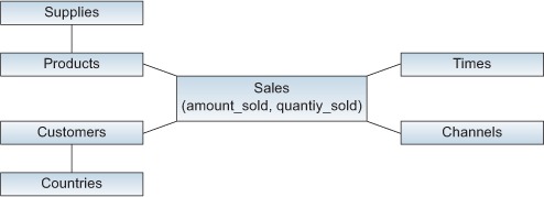
Figure 3.7. Sales fact as a star. All supplier attributes are included as additional columns in the products dimension. All country information is included in the customers dimension as additional columns. The database only needs to optimize one join for the relevant information.

Figure 3.8. Sales fact as a snowflake. The relevant supplier information has been normalized out of products. The database needs to join to the suppliers table from the products table to be able to aggregate and group by supplier attributes.

When is using a snowflake design a good idea? There are typically two use cases where snowflakes make good sense:

• To reduce the size of dimension tables by factoring out seldom used but really big columns —Most product data, such as categories and types, are small 10- to 250-character fields, but what if there’s a very large (CLOB or LARGETEXT) field that includes a very long product description? It’s possible that this needs to be included in Mondrian for some reports but that it’s not a commonly used column. Keeping it in the same table, for a row-store database, means the database may be doing a bunch of unnecessary I/O. In short, you might be able to speed up the most common queries that don’t use that column by factoring out a handful of columns into a separate table.
• To more easily manage a Type I type attribute in an otherwise Type II dimension —Consider the snowflake design in figure 3.8, where we’ve factored out countries from customer. It’s likely that many customer attributes will change over time (including which country the customer lives in) and will need to be managed as Type II dimensions. The attributes of the country, however, such as its name, tend to be Type I changes when they happen (updates, without any history). Using a snowflake design to separate out a table with update instead of change-tracking attributes allows for easy Type I updates in an otherwise Type II dimension.

3.2.4. Degenerate and combination/junk dimensions

There are times when creating a whole separate dimension table, including a foreign key reference, and then grouping by attribute just doesn’t make sense for performance reasons. For instance, when the dimension only has a single attribute (such as order type or channel), it’s overkill to create another join path, a separate table for housekeeping, and so on for simple attributes. There are also times when you’d like to include attributes that aren’t really analytically significant, but that are nice for drilling and for including on some drill-through reports. For example, the original order ID for an order would be nice to keep around, so that you could include it on a report to find exceptions or to look up outliers in the original source system. Again, including that as a standard dimension would be impractical because the number of rows in the original order ID dimension would grow close to the same millions of records in the fact table. We’ll cover the common techniques for addressing these challenges: degenerate dimensions and combination (or junk) dimensions.

Consider our sales fact example, which includes a few low ordinality items. We have a sales type attribute that has very low ordinality (two different values), indicating what type of sale record this is: NEW or RETURN. We also have a channel type (INTERNET or RETAIL) that is similar. We also want to keep track of an order ID, which will cause a very large dimension (nearly as large as the fact). (See figure 3.9.)

Figure 3.9. Modeled as standard dimensions using surrogate foreign key references and joins. The sales type dimension includes only two records, as does channel dimension. The original order dimension includes nearly as many rows as the fact table does because every new order also needs a new record in the order dimension.

For the single attribute dimensions (channel and sales type) it seems overkill to maintain entire dimensions with only single-attribute, low-ordinality dimensions. We can include these attributes as columns directly in the fact table, eliminating the separate table and additional join entirely. This is the ultimate in denormalizing, where the attribute is kept directly with the fact. Mondrian can be configured so that columns in the fact table still show as a separate dimension, but will use the columns directly from the fact table without doing any additional joins (figure 3.10).

Figure 3.10. Channel, sales type, and original order included as degenerate dimensions in the fact table. This makes sense for small, single-attribute dimensions, where it’s beneficial to eliminate management for a separate dimension and eliminate unnecessary joins to very small (or very large in the case of the original order) dimensions.

We can eliminate the joins and manage the attributes for those dimensions directly in the fact table. This only works for small, low-ordinality columns or very large high-growth attributes that grow with the fact table.

What happens when you’ve included a bunch of these low-ordinality, single-attribute dimensions in the fact table? A couple of attributes are usually OK, but when you have a bunch of longer (10- to 50-VARCHAR) fields, your fact table size will likely be growing more than you’d like (compared to just using dimension integer surrogate keys). There’s another technique for taking lots of single-attribute degenerate dimensions, and putting them back into a standard dimension of unrelated attributes. This type of dimension is referred to as a combination dimension, or commonly as a junk dimension. It should be noted that the only reason to do this is for performance; from Mondrian’s perspective, assuming it’s been configured properly, there’s no logical difference between consolidating multiple degenerate dimensions into a junk or combination dimension and leaving them as degenerate dimensions in the fact table (figure 3.11).

Figure 3.11. Multiple unrelated degenerate dimensions (channel, sales type) can be consolidated into a junk dimension. This provides the performance benefits of a small, single integer in the fact table and reduces the size of the fact table. Note that the high-ordinality degenerate dimension (original order) isn’t moved into the junk dimension because to do so doesn’t make sense.

Junk dimensions are created in a unique way: a Cartesian product of all possible combinations of attributes is created, along with a surrogate key. Then, when you’re loading the fact table, the loading process looks into the junk dimensions to grab the record with the correct set of attributes (for example NEW, INTERNET is record 100), which is guaranteed to be in the dimension because all possible combinations are present.

-- All possible combinations of attributes (Channel/Sales Type)
-- are created, along with a surrogate
select * from junk_dim;
+-------------+--------------+------------+
| junk_dim_id | channel_name | sales_type |
+-------------+--------------+------------+
|         100 | INTERNET     | NEW        |
|         101 | INTERNET     | RETURN     |
|         102 | RETAIL       | NEW        |
|         103 | RETAIL       | RETURN     |
+-------------+--------------+------------+

3.3. Summary

In this chapter, we looked at how data should be structured for use by Mondrian in analysis. You saw how and why data is extracted from operational, normalized databases, enriched, and put into a star schema. We also discussed some of the architectural characteristics of an analysis database. Finally, we took a look at some advanced concepts in dimensional modeling.

Now that we’ve covered the basics of the star schema, some of its ins and outs, and the overall architecture, we’re ready to configure Mondrian on top of the star schema. The next chapter will show you how to bring together the physical star schema and the logical analytic structures to create a complete solution. You really should have a good sense of the basics of star schema design, and most importantly the splitting of attributes into facts and dimensions, along with the foreign key patterns we outlined in this chapter, before continuing.