Chapter 4. Multidimensional modeling: making analytics data accessible

This chapter is recommended for

	Business analysts
	Data architects
	Enterprise architects
	Application developers

In chapter 2, you saw how business questions could be described by creating cubes, dimensions, attributes, and measures, and how a schema contains those logical elements. Then, in chapter 3, you saw how to design and populate the data warehouse.

Mondrian uses the concept of a schema to map from the logical data structure used for analysis to the physical structure used in the data warehouse. A completed schema provides cubes that can be used for data analysis. In this chapter, you’ll see how to build a schema. (It’s a long chapter, because no matter how you slice it, multi-dimensional modeling is a dense topic. We suggest you read the first section, and then take a break before you proceed with section 4.2.)

This chapter describes the XML grammar of Mondrian schemas and the key XML elements and attributes. You’ll see in detail not only how to define the logical elements (cubes, dimensions, attributes, and measures) used in analytics, but also how to map them onto physical data structures (tables and columns) so that Mondrian knows how to get the data from the data mart.

You’ll see how to create a simple cube with a couple of dimensions and measures, and then you’ll see how that cube can be extended, adding more dimensions, navigation hierarchies, and calculations. In chapter 5, we’ll cover some more advanced topics in schema design, building on the material in this chapter.

This chapter is essential if you’re an architect designing a Mondrian schema. It assumes that you’re familiar with XML, as well as the material covered in the previous chapters. If you’ll be using prebuilt Mondrian cubes, however, and you’re an analyst defining reports and dashboards, you can probably skip this chapter and the next one.

We’ll start with a simple example showing the absolutely essential elements: Schema, Cube, Dimension, Attribute, and Measure. Later in this chapter, and continuing on in chapter 5, we’ll describe other important schema elements, interspersed with explanations and examples. We’ll cover almost all XML elements and their important attributes, but these chapters are not meant to be exhaustive. The online Mondrian documentation contains the definitive reference to all 80 XML elements in a Mondrian schema.

A brief word about how names appear in the text. As we discuss various schema features and define example schemas, we shall refer in the text to the objects in those schemas, and their names appear in code font with the parts of the name enclosed in brackets, as if you were using the object in an MDX query. For instance, a measure named “Unit Sales” would appear like this: [Measures].[Unit Sales]. The MDX language does not require brackets if the parts of the name contain only letters, but we use brackets throughout for consistency.

4.1. A simple schema

Section 2.3 described a company building a report to improve its sales process. The report compared sales to customers with a college education this year to last year. In order for Mondrian to run that report, you need to define the cube that the report is based on, and how that cube is mapped onto the data mart. A schema is what provides those definitions.

Figure 4.1 shows the elements defined in that schema and an outline of the XML schema file. Listing 4.1 shows the XML schema in full. Don’t be concerned with understanding each of the elements in the schema at this point; rather, focus on the overall composite of information contained within a typical Mondrian schema.

Figure 4.1. Sales schema mapped to an XML schema outline

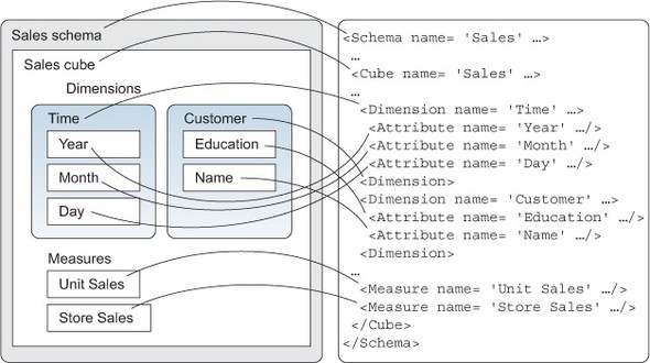
Listing 4.1. Sales schema

Because this is the first schema in this book, we’ve listed it in its entirety. There are quite a few XML elements, but it’s not important to understand them all right now. At first, we’ll only cover the key elements: Schema, Cube, Attribute, Dimension, Measure, and PhysicalSchema. The following sections will discuss each of these elements.

The other elements will be described later in the chapter: MeasureGroups, MeasureGroup, Measures, DimensionLinks, and ForeignKeyLink.

4.1.1. Schema element

The Schema XML element is the top-level element of a Mondrian schema. There is one, and only one, Schema element in a Mondrian schema XML file, and it represents the container for all the pieces the schema contains. An analyst would first create a schema and then fill in all the attributes, dimensions, and cubes that together address the business questions.

<Schema name="Sales"
  caption="Sales"
  description="Optimizing the Sales process at Two Wheels Cycles"
  metamodelVersion="4.0" measuresCaption="Measures"
  defaultRole="Associate" missingLink="warning">

Each schema must have a name attribute (although Mondrian doesn’t do anything important with that name), and we recommend that you also provide a description.

We also recommend that you specify metamodelVersion="4.0", because it helps with schema versioning ("4.0" is the current version of Mondrian, and likely the version for which you’ll be writing your schema).

Because Schema is the sole root element in the XML document, it contains all of the top-level elements that constitute the schema. A schema always includes a PhysicalSchema element, and it generally includes one or more Cube elements. Other common elements include Dimension (to define public dimensions—dimensions shared between cubes), and Role for access control.

Ordering of XML elements

In previous versions of Mondrian, the schema parser was extremely sensitive about the order of child elements. If you got child elements in the wrong order (for example, a cube after a role, instead of before as Mondrian was expecting), Mondrian would silently ignore the cube. This situation has been fixed in Mondrian version 4.0. If you’ve used previous versions of Mondrian, this is one thing you can stop worrying about!

4.1.2. Cube element

A cube, defined by a Cube XML element, is the context for a report or interactive analysis session. It represents a collection of events, describing the occurrences of a particular business process over the lifetime of the data warehouse. The collection may contain a large number of events—thousands, millions, or even billions—but the events are not presented individually.

Cubes tend to be a complete set of measures and attributes for doing an analysis on the set of events. For instance, if you’re interested in sales by customer attributes, you might want to look at sales amounts (events or measures) by customer geography (attributes). A cube collects these things into one place, ready for analysis and querying.

A cube has little configuration itself, but is instead mostly an element that holds the more important measure groups and dimensions. There is usually, but not always, a one-to-one relationship between a star schema (a single fact table and dimension tables outlined in chapter 3) and a cube (measures and dimensions). (For instance, the analyst in chapter 2 would likely have built a star schema containing a sales fact table and customer dimension table to store the data for the [Sales] cube and its [Customer] dimension.)

<Cube name="Sales">
  <Dimensions>
    ...
  </Dimensions>
  <MeasureGroups>
    ...
  </MeasureGroups>
</Cube>

Recall from chapter 2 that a cube is a collection of measures and attributes. The measures quantitatively describe events or collections of events, and the attributes represent the context in which the events occurred. By choosing appropriate measures and attributes, a business user can focus on the part of the history that answers their question. Each combination of attributes and measures is effectively a new report that can be created in seconds using a point-and-click interface, and there’s an exponential number of such combinations.

In the XML syntax, there are intervening XML elements between the cube and its constituent attributes and measures. Attribute elements occur within Dimension elements, and all dimensions in a cube are within a Dimensions element. Measure elements occur within a MeasureGroup element, and this is inside a MeasureGroups element. Cubes that contain multiple measure groups are a fairly advanced topic that we’ll revisit later in section 5.1.5); we’ll explain dimensions shortly (in section 4.1.4).

4.1.3. Attribute element

An Attribute XML element describes a data value. If you’re familiar with modeling relational database schemas, an attribute is the nearest equivalent in the Mondrian schema to a column. In practice, nearly all of the columns in your dimension tables (see section 3.1.3) will be configured via attribute elements.

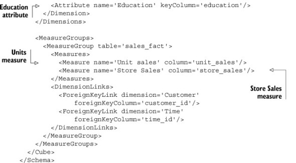
In the [Sales] cube (see figure 2.10) one of the attributes to be analyzed is the education of the customer. This will likely be a column (education) in a dimension table (customers) in the database star schema, and also a configured XML Attribute element.

<Attribute name="Education" caption="Education level"
    description="The education level of this customer"
    keyColumn="education"/>
<Attribute name="Name" keyColumn="customer_id" nameColumn="full_name"/>

The preceding example shows the [Name] and [Education] attributes from the [Customer] dimension. Every attribute must have a name. The [Education] attribute has, in addition, caption and description attributes.

Name, caption, and description

Captions are similar to names, and people often confuse the two. The purpose of a caption is to be displayed on the screen to a business user, whereas the name is intended to be used in code, particularly in an MDX statement.

Often the name and caption are the same (and the caption defaults to the name if a caption is not explicitly specified). But they have different localization behavior: captions can be localized, but the name is the same in all languages. This makes sense, when you consider that your business users will expect to see captions on the screen in their own language, whereas the underlying MDX code needs to be the same regardless of the language the client is using.

For example, here’s an attribute whose caption and description have been localized into French:

<Attribute name="Marital Status" caption="Etat civil"
  description="L'état civil de ce client" keyColumn="marital_status"/>

You use its name, [Marital Status], when writing MDX:

SELECT ... ON COLUMNS,
   [Customer].[Marital Status] ... ON ROWS
FROM [Sales]

but as figure 4.2 shows, the attribute is labeled in French (“Etat Civil”) when the query results appear in a user interface.

Figure 4.2. Report showing localized caption

Descriptions are quite straightforward. Many user interfaces (such as Pentaho Analyzer and Saiku) display descriptions as tooltips when you move the mouse over an element. Descriptions can help business users find their way around a cube that they’re unfamiliar with. Like captions, descriptions can be localized.

Name, caption, and description are not unique to attributes; the other elements that may appear on business user’s screen also have them, including Schema, Cube, Measure, and Dimension. They also have a visible attribute, which tells the user interface to hide the element but doesn’t affect its behavior in MDX queries. To see which elements have name, caption, description, and visible attributes, consult the Mondrian online documentation. (Appendix B lists all online resources.) The same localization rules apply: caption and description can be localized; name can’t be, and is therefore the same for all locales.

Mapping attributes onto columns

We said that an attribute is like a column, but because attributes are part of a dimensional model intended for business users, the behavior is richer. Every attribute is based upon at least one database column. For example, [Education] is a simple attribute that’s mapped, via the keyColumn attribute, onto the education column of the customers table.

For each property of an attribute, you can specify the property using an XML attribute, or there’s an equivalent nested XML element. Table 4.1 shows the elements and attributes available.

Table 4.1. XML elements and attributes that map dimensional attributes onto columns

XML attribute	Equivalent nested XML element	May be composite?	Description
keyColumn	Key	Yes	Required. Specifies the column that holds the key for members of this attribute. The key must be unique.
nameColumn	Name	No	Optional. Specifies the column that holds the name of members of this attribute. If not specified, it defaults to the key (or the last key column if the key is composite).
orderByColumn	OrderBy	Yes	Optional. Specifies sort order. If not specified, attribute is sorted by key.
captionColumn	Caption	Yes	Optional. Defaults to name, which in turn defaults to last column of key.

Table 4.2 shows example attributes, illustrating cases where it makes sense for the attribute’s name, caption, and ordinal to be different from the attribute’s key.

Table 4.2. Example attributes

Dimension	Attribute	Key	Name	Caption	Ordinal	Comments
Time	Year	2012	2012	2012	2012	Same value for all properties.
Time	Month	[2012, 1]	1	January	[2012, 1]	Composite key ensures that January 2012 is distinct from January 2011. Name is distinct from caption; thus the unique name is [Time].[2012].[1], but “January” is displayed on the screen (in applications running in the English locale).
Customer	Name	13874	Bob Arctor	Bob Arctor	[Arctor, Bob]	Numeric key ensures uniqueness if there happen to be two Bob Arctors. Caption is same as name, because attribute is not localized. (It is unusual for attributes with large numbers of distinct values to be localized.) Composite ordinal sorts customers by their last name.
Customer	State	[USA, CA]	CA	CA	[USA, CA]	Key is composite, because the same state name may occur in different nations.

4.1.4. Dimension element

A Dimension is a collection of logically related attributes. If, as we said earlier, an attribute is the dimensional equivalent of a column, then a dimension is the equivalent of a table. (And, in fact, many dimensions map directly to a dimension table in the star schema.)

What do we mean by logically related? [Gender], [Zipcode], and [State Population] belong in the [Customer] dimension because they are all properties associated with the customer who made a particular purchase. [Day of Week] belongs in the [Time] dimension, not the [Customer] dimension, because it does not depend on the customer: a customer might have one purchase on a Monday in their history and another on a Thursday.

There’s also a more down-to-earth reason to group attributes into dimensions. If a cube contains a large number of attributes, dimensions are a convenient way of grouping them on the screen, in the same way that folders make large numbers of files easier to manage.

4.1.5. Measure element

The Measure XML element defines a measure. A measure is a value, almost always numeric, that appears in a cell. If the cell represents many rows in the fact table, then the cell’s value is the measure aggregated (usually summed) over all of those rows. Measures are the aggregated values from columns in the fact tables described in chapter 3; they represent the what you’re trying to measure.

Consider the cell showing the [Unit Sales] measure in the second row of figure 4.2, with a value of 12. This means that 12 units were sold to customers whose country was France and whose marital status was M. There happen to have been three sales transactions, therefore three rows in the fact table, with those criteria, and their values in the unit_sales column are 3, 1, and 8. The cell value, 12, is the sum of these values.

Strictly speaking, the XML Measure element defines a stored measure. Mondrian also supports calculated measures, which are calculated from other measures using an MDX formula. Though stored and calculated measures are defined and evaluated differently, they appear the same to a business user running a report. Calculated measures, and more generally calculated members, are described in section 5.4.2.

Here are some measures:

<Measure name='Unit Sales' aggregator='sum' column='unit_sales' />
<Measure name='Store Sales' aggregator='sum' column='store_sales' />
<Measure name='Sales Count' aggregator='count' />

Each measure has a name and an aggregator, describing how to roll up values. Table 4.3 shows the available aggregators. A column attribute describes which column’s values are to be aggregated; it’s required for all aggregators except count. A count measure without a column, such as the [Sales Count] measure in this example, counts rows.

Table 4.3. Aggregators

Aggregator	Comments
sum	Sums numeric values. The most common aggregator.
count	Counts the number of rows for which a column is not null; if column isn’t specified, counts the number of rows.
distinct-count	Computes the number of distinct values of the column. Nulls are not counted.
max	Finds the maximum value of a column.
min	Finds the minimum value of a column.
avg	Computes the average value of a numeric column.

Aggregate functions in Mondrian and SQL

If you’re familiar with aggregate functions in SQL, then Mondrian’s aggregate functions will look familiar. Each aggregator maps to a SQL aggregate function in an obvious way. For instance, the [Unit Sales] measure becomes SUM(unit_sales) in generated SQL, and [Sales Count] becomes COUNT(*).

Like other elements that appear in a report, a measure definition also includes caption, description, and visible attributes.

4.1.6. PhysicalSchema element

The PhysicalSchema XML element describes which tables and columns in the data mart provide the data for the dimensions and cubes in the schema. The physical schema is not something that the business user is aware of; the business user interacts only with the logical model (cubes and dimensions).

The physical schema is a close representation of the physical star schema, with the fact table and dimension tables, their columns, data types, and relationships. You’d expect most of the columns, including the surrogate IDs for Slowly Changing Dimensions (covered in section 3.2.1) and foreign keys in your fact table, to be defined in your physical schema.

The purpose of the physical schema is to provide a foundation for building the logical model. As figure 4.3 shows, the physical schema is a bridge between the logical model and the actual database. It presents a simple model of tables, columns, and links between tables, where the reality may be more complex. For example, a “table” in the physical schema may really be a view or a SQL query. Two tables with different names might be uses of the same database table, or may inhabit different schemas or different database instances. A column with data type “integer” might actually have a data type of NUMBER(10, 0) when stored in Oracle.

Figure 4.3. Logical and physical schemas

The physical schema also allows the structure of the data mart to change over time. For instance, suppose that a table you need as a fact or dimension table doesn’t exist in the schema but can be computed using a SQL query. You can create a placeholder “table” in the physical schema and run queries against it. Tomorrow, when you have fixed the ETL process to create and populate a real table, you can change the physical schema to use the real table; you won’t have to change the logical schema, because the physical schema has insulated rest of the model from changes to table structure.

The physical schema shown in figure 4.4 and in listing 4.2 declares tables customer, time_by_day, and sales_fact. It declares primary keys for customer and time_by_day, which are needed because these tables will contain dimensions; sales_fact is a fact table, so it doesn’t require a primary key. No columns are defined, so Mondrian reads each table’s column definitions from JDBC.

Figure 4.4. Physical schema of the Sales data mart

Listing 4.2. Physical schema

Inside each table, you can list the columns explicitly. As well as serving as a check that the columns your schema needs still exist in the database, this allows you to specify a precise type. You can also define calculated columns.

Listing 4.3 includes three columns customer_id, fname, and lname, and it defines a calculated column, full_name, by concatenating first name and last name. Note that when the fname and lname columns are used in the expression for full_name, we use the <Column> element, because we’re using, not defining, a column.

Listing 4.3. Physical schema with columns

When Mondrian generates a SQL query to retrieve data from the database, it’ll generate an expression based on the formula within the SQL element, replacing the Column elements with references to other columns.

One problem with SQL is that database dialects tend to differ significantly. The schema we just wrote will work on Oracle and PostgreSQL, which use the conventional || operator for concatenating strings, but it will fail on MySQL, which uses the CONCAT() function. Is it possible to write one Mondrian schema that will work against multiple SQL databases?

Yes! The ExpressionView element allows multiple SQL child elements, with a dialect attribute to distinguish them. When you add support for MySQL, a fragment of the previous listing becomes what’s shown in listing 4.4.

Listing 4.4. Calculated column with expressions for multiple SQL dialects

Each table in a physical schema has a unique alias, and the alias defaults to the table name. Usually you don’t need to assign a table an alias, but the following listing shows some exceptions.

Listing 4.5. Table alias examples

Why would you want to create more than one use of the same table? Usually to avoid ambiguities in join paths. For example, consider a movie database where a film has both a language and an original language; the language is usually the same as the original language, but it will be different if the film is dubbed. The Film dimension has one use of the film table and two uses of the language table, via different foreign keys. When defining the physical schema, you’d create a link between the film table and each use of the language table, as shown in listing 4.6.

Listing 4.6. Multiple uses of the same table

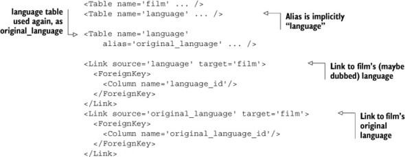
When you base an attribute on a column in either the language or original _language table in the physical schema, it’s clear which join path is intended.

Putting it together

PhysicalSchema is the last of the elements you need to build a simple multidimensional schema. It defines the tables and relationships between them. Upon these, you can build a cube, which contains dimensions, attributes, and measures. A cube is the unifying concept that allows business users to analyze their own data.

In this section, you’ve seen how to build a simple cube. Next, we’ll look at the overall structure of a schema file, and at some of the more advanced concepts it supports.

4.2. Anatomy of a schema

Now you’ve seen an example of a schema file and some background on its structure and purpose. Why are schema files defined in XML? What tools can be used to author a schema? What are the valid contents of a schema? That’s what we’ll look at in this section.

4.2.1. XML schema files

Why does Mondrian use XML as the language to define schemas? By design, Mondrian gives people a choice about whether they’ll author schemas with a tool (such as Schema Workbench) or with a text editor. XML is a language that can be written and read by both humans and computers, and the particular dialect of XML used is designed to be concise to type and forgiving of errors.

XML also improves interoperability between tools. For example, the Pentaho Aggregate Designer generates fragments of XML and inserts them into a schema. And, you can achieve some powerful effects by writing a dynamic schema processor, which is invoked as a connection is being created, reads the source XML schema, and transforms it to another piece of XML. Dynamic schema processors are used for applications such as localization and access control in a multi-tenant environment. They’re described in section 8.2.

Mondrian schemas can be processed with standard text-processing tools such as grep and diff. Authoring tools are encouraged not to make wholesale changes to the XML, because this makes it difficult to store schemas in a version-control system, such as Subversion or git.

XML elements typically have quite a few attributes and subelements, but we won’t describe all of them here. This chapter aims to describe the general purpose of each XML element, but the definitive description of each element is in Mondrian’s online schema reference, as described in appendix B. We sometimes describe attributes separate from their parent element, where it makes logical sense. For example, we discuss the Schema element’s defaultRole attribute when we discuss roles and access control in chapter 6.

4.2.2. Structure of a schema

Figure 4.5 shows the elements allowed in a Mondrian schema and their hierarchical structure.

Figure 4.5. Hierarchical structure of a Mondrian schema

As you’ve seen, Schema is always the root element. In the simple schema, its children were a PhysicalSchema and a Cube; children can also include more Cube elements and also Dimension, Role, NamedSet, UserDefinedFunction, Parameter, and Annotations elements.

Some elements can occur in more than one context. For instance, Dimension may occur within a cube (when defining a private dimension), or it can be a child of a schema (when defining a shared dimension, as you’ll see in section 5.1.2, in the next chapter).

Some elements exist to hold a collection of child elements of the same type. These are called holder elements. A holder element doesn’t have attributes, and its name is the plural of the name of the element it contains. For example, the Dimensions element contains a list of Dimension elements. Other examples include Columns, Dimensions, Hierarchies, and Attributes.

Some holder elements’ children have types that are similar but not identical. For example, DimensionLinks has children ForeignKeyLink, FactLink, ReferenceLink, and NoLink. These elements have a similar purpose—to create a link between a dimension and a measure group—and several attributes in common.

4.2.3. Schema versioning and upgrading

We recommended earlier that you include the metamodelVersion="4.0" attribute in your Schema element. This is necessary because Mondrian’s schema language changes over time. Each Mondrian release introduces new concepts, and these are manifested as new XML elements and attributes. The version number allows the Mondrian engine to decide whether to run the schema as is, or to try to upgrade automatically.

The version number is particularly important in the version 4.0 release because there was a major change in the schema metamodel between Mondrian versions 3.x and 4.0. The Mondrian 4.0 engine is able to upgrade most 3.x schemas automatically. For example, Mondrian 3.x virtual cubes became obsolete in Mondrian 4.0, and Mondrian automatically converts each VirtualCube element to a cube that has multiple MeasureGroup elements.

The metamodelVersion attribute was only introduced in version 3.4.2, and using it is strongly recommended from version 4.0 onward. If the attribute is missing, Mondrian will do its best to guess the intended target version. (If there’s a PhysicalSchema element, Mondrian assumes that the schema was intended for version 4.0 but the author forgot the version attribute; otherwise Mondrian assumes that the schema is in 3.x format.)

The metamodelVersion attribute will allow future versions of Mondrian to upgrade schemas, and will also allow Mondrian to detect a schema that is too recent. For example, if there are significant changes to the schema in Mondrian 5.0, a schema written for that engine will be stamped with metamodelVersion="5.0" and the Mondrian 4.0 engine will refuse to run it.

Now you’ve seen a simple schema and we’ve covered the overall structure of a schema file. For the remainder of the chapter, we’ll look at the elements that allow you to slice and dice data: dimensions and attributes, hierarchies and levels.

4.3. Dimensions, hierarchies, and levels

Multidimensional analysis is a top-down technique. Rather than looking at individual rows, an analyst often starts off by looking at a single row that summarizes the entire dataset, and then zooming in on the data of interest. You saw already how attributes allow you to subdivide the dataset into groups, or to winnow the data into a smaller group. Now we’ll look at how organizing attributes into hierarchies and levels allows a business user to navigate more intuitively and efficiently.

Each analyst knows that their business users naturally arrange data into these hierarchies; a year is composed of four quarters, and quarters are composed of three months. And the users want to examine their measures up and down different levels of aggregations. This section will help make your schema reflect the reality of these relationships that your users already know and want.

Then we’ll look more closely at the most familiar dimension of them all, the time dimension. You’ll see that there are some deep unifying patterns within the dimensional model, that measures are members of their own special dimension, and that every attribute has its own hierarchy, whether or not it is organized into a multi-level hierarchy.

4.3.1. Hierarchies and levels

You’ve seen how you can use attributes to qualify the data shown in a report, and how attributes are organized into dimensions. The attributes of a dimension can always be used independently, but some attributes are so closely related that most users will want to use them together. To do this, you can define a hierarchy.

Listing 4.7 builds a hierarchy called [Customers] from the attributes [Country], [State], and [City]. These attributes form the three levels of the hierarchy.

Listing 4.7. Customers hierarchy

<Dimension name='Customer'>
  <Attributes>
    <Attribute name='Country' ... />
    <Attribute name='State' .../>
    <Attribute name='City' .../>
  </Attributes>
  <Hierarchies>
    <Hierarchy name='Customers'>
      <Level attribute='Country'/>
      <Level attribute='State'/>
      <Level attribute='City'/>
    </Hierarchy>
  </Hierarchies>
</Dimension>

Figure 4.6 shows some of the members of the hierarchy.

Figure 4.6. Members of the Customers hierarchy

Hierarchies allow for a better experience in the user interface. For example, the members of a hierarchy can be displayed in a single column, rather than with one column for each level; each member is preceded by a “+” or “-” icon, allowing it to be expanded or collapsed. Several navigation actions are possible if a member belongs to a multilevel hierarchy. Double-clicking on the [California] member might drill down, so that the axis now consists of just the cities in California. Another action supported by many user interfaces is drilling up: [California] would be replaced by the nations [Canada], [Mexico], and [USA].

That said, sometimes a hierarchy is too restrictive. For a particular analysis, the business user might wish to show only certain levels of the hierarchy, or to put one level on the columns axis and another on the rows. The best practice is to design a schema with just the attributes at first; then create hierarchies to optimize common navigation paths between attributes, but leave the attributes visible so that business users can work with the raw attributes if they prefer.

The attribute of each level of a hierarchy must have a strict one-to-many relationship with the attribute of the next level. In the [Customers] hierarchy, each state belongs to only one country, and each city belongs to only one state. The net effect is that each level down has more members than the last.

If your attributes don’t have this structure, you probably shouldn’t be creating a hierarchy on them. Consider, for example, the [Month] and [Week] attributes of a [Time] dimension, as shown in table 4.4.

Table 4.4. Month and Week attribute values

Year	Month	Week	Day of week	Day
2012	January	4	Saturday	28
2012	January	5	Sunday	29
2012	January	5	Monday	30
2012	January	5	Tuesday	31
2012	February	5	Wednesday	1
2012	February	5	Thursday	2
2012	February	5	Friday	3
2012	February	5	Saturday	4
2012	February	6	Sunday	5

Week 5 of 2012 straddles both January and February of 2012. The relationship between [Month] and [Week] is therefore many-to-many, not one-to-many as required for a hierarchy. The member for week 5 of 2012 does not have a well-defined parent, so you can’t define a hierarchy where [Month] is the parent level of [Week].

Keeping Weeks from Crossing Year Boundaries

Time dimensions often have two time hierarchies defined: Year-Month-Day and Year-Week-Day. To prevent weeks from crossing year boundaries, years often start with a shortened week 1 and end with a shortened week 53.

But hold on! Both January and February contain a member whose [Day] value is 1. Surely this breaks the rule that a member can have only one parent. No, because January 1, 2012, and February 1, 2012, are different members. They may both have the name [1], but their keys are different (Julian dates 2455927 and 2455958, respectively). The short-form name is more convenient to display, and it’s unique provided that the member is shown in the context of its parent month. (The concise name is, in fact, another good reason to use a hierarchy.)

Note what has happened here. Organizing attributes into a hierarchy doesn’t affect the number of instances of that attribute. The [Day] attribute has 365 (or 366) distinct values for each year covered by the [Time] dimension, and the resulting [Day] level has the same number.

So, when defining an attribute, you need to define a key that gives the attribute enough distinct values. The attributes of the [Time] dimension show the various approaches:

<Attribute name='Year' keyColumn='year'/>
    <Attribute name='Month'>
      <Key>
        <Column name='year'/>
        <Column name='month_of_year'/>
      </Key>
    </Attribute>
    <Attribute name='Week'>
      <Key>
        <Column name='year'/>
        <Column name='week_of_year'/>
      </Key>
    </Attribute>
    <Attribute name='Day' keyColumn='date_id'
        nameColumn='day_of_month'/>

Schema shorthands

The previous example used them, so now is a good time to discuss the topic of schema shorthands. XML can be quite a verbose language, which is fine if a machine is generating the XML (in order to save the state of a graphical schema design tool, for instance), but it’s not as good if you’re writing the XML by hand in a text editor. Mondrian allows common constructs to be expressed more concisely.

In the previous example, the [Year] attribute could have been written as follows:

<Attribute name='Year'>
  <Key>
    <Column name='year'/>
  </Key>
  <Name>
    <Column name='year'/>
  </Name>
</Attribute>

But we abbreviated that to keyColumn='year' because the key has just one column and the name is the same as the key.

The [Month] attribute in the previous example is equivalent to the following:

<Attribute name='Month'>
  <Key>
    <Column name='year'/>
    <Column name='month_of_year'/>
  </Key>
  <Name>
    <Column name='month_name'/>
  </Name>
</Attribute>

That’s because the name of a composite key is by default the last component of that key (the month_of_year column in this case).

There are other shorthands. If you’re writing XML by hand, learn the available shorthands and save yourself some typing! The full set of schema shorthands is in the online Mondrian documentation.

Disconnected attributes

We just described how to ensure that the [Month] attribute has 12 values per year (120 values if your time dimension contains 10 years), but what if you wanted to compare sales that happened from any January to any December? You’d want a version of the month attribute that has 12 values; January would contain sales that happened in any January, and so forth.

In this case, you’d define an attribute for which the year column is not part of the key:

<Attribute name='Month of Year' keyColumn='month_of_year'
    nameColumn='month_name'/>

There is no formal relationship between this [Month of Year] and the [Month] attribute defined previously, but because the attributes are grouped into the [Time] dimension and are similarly named, your users will figure it out.

4.3.2. Time dimension

Cubes almost invariably have a time dimension. In section 3.2.2, you saw why it was a good idea to model time dimensions as Type I dimensions: a time dimension table containing one row for each day in the dataset, a surrogate key (usually an integer) containing the day ID, and a foreign key column in the fact table referencing that key. One of the advantages of that approach is that the time dimension is modeled much like any other dimension: there’s a collection of attributes that can be used individually or organized into hierarchies.

MDX contains a number of operators specific to the time dimension (see table 4.5). For example, the YTD (year-to-date) function generates a range of members between the start of the year and the current time member; summing over these members yields a running total:

WITH MEMBER [Measures].[Unit Sales to Date] AS
  Aggregate(YTD(), [Measures].[Unit Sales])
SELECT {[Measures].[Unit Sales],
        [Measures].[Unit Sales to Date]} ON COLUMNS,
 [Time].[1997].Children ON ROWS
FROM [Sales];

|           | Unit Sales | Unit Sales to Date |
+------+----+------------+--------------------+
| 1997 | Q1 |     66,291 |             66,291 |
|      | Q2 |     62,610 |            128,901 |
|      | Q3 |     65,848 |            194,749 |
|      | Q4 |     72,024 |            266,773 |

Table 4.5. MDX time operators

Function	Description
YTD() or YTD(member)	Year to date
QTD() or QTD(member)	Quarter to date
MTD() or MTD(member)	Month to date
WTD() or WTD(member)	Week to date

To enable these operators, you need to tell Mondrian which attributes represent which kind of time period using Dimension’s type attribute and Attribute’s levelType attribute. Listing 4.8 shows how these attributes are used.

Listing 4.8. Labeling a time dimension and its attributes

Time dimension table generator

The most common way to generate a time dimension table is through an ETL tool. Pentaho Data Integration, for instance, includes a Time Dimension generator in its examples directory that can be used piecemeal or can be enhanced to build time dimension tables. But sometimes a tool like this isn’t available, such as when you’re running Mondrian against an operational schema. Mondrian provides a neat way to generate and populate a time dimension the first time you need it.

Recall how you declare a regular time dimension table:

<PhysicalSchema>
    <Table name='time_by_day'/>
    <!-- Other tables... -->
</PhysicalSchema>

Mondrian sees the table name, time_by_day, checks that it exists, and finds the column definitions from the JDBC catalog. The table can then be used in various dimensions in the schema. An auto-generated time dimension is similar:

<PhysicalSchema>
    <AutoGeneratedDateTable name='time_by_day_generated'
        startDate='2012-01-01' endDate='2014-01-31'/>
    <!-- Other tables... -->
</PhysicalSchema>

The first time Mondrian reads the schema, it notices that the table isn’t present in the schema, and it creates and populates the table. Here’s the DDL:

CREATE TABLE `time_by_day_generated` (
  `time_id` Integer NOT NULL PRIMARY KEY,
  `yymmdd` Integer NOT NULL,
  `yyyymmdd` Integer NOT NULL,
  `the_date` Date NOT NULL,
  `the_day` VARCHAR(20) NOT NULL,
  `the_month` VARCHAR(20) NOT NULL,
  `the_year` Integer NOT NULL,
  `day_of_month` Integer NOT NULL,
  `week_of_year` Integer NOT NULL,
  `month_of_year` Integer NOT NULL,
  `quarter` VARCHAR(20) NOT NULL);

The table contains one column for each time domain (shown in table 4.6). Table 4.7 shows the first few rows generated.

Table 4.6. Time domains recognized by <AutoGeneratedDateTable>

Role	Default column name	Default data type	Example	Description
JULIAN	time_id	Integer	2454115	Julian day number (0 = January 1, 4713 BC). An additional attribute, epoch, if specified, changes the date at which the value is 0.
YYMMDD	yymmdd	Integer	120219	Decimal date with two-digit year.
YYYYMMDD	yyyymmdd	Integer	20120219	Decimal date with four-digit year.
DATE	the_date	Date	2012-12-31	Date literal.
DAY_OF_WEEK	day_of_week	Integer	2	Ordinal of the day of the week: a value from 1 to 7. The first day of the week varies by locale. In the U.S. it’s Sunday; in France it’s Monday.
DAY_OF_WEEK_NAME	the_day	String	Friday	Name of day of week.
DAY_OF_WEEK_IN_MONTH	day_of_week_in_month	Integer	1	Ordinal number of the day of the week within the current month. For example, the third Friday of the month will have the value 3. Unlike DAY_OF_WEEK, the value is the same in all locales. Days 1 through 7 of a month have the value 1, days 8 through 14 are 2, and so forth.
MONTH_NAME	the_month	String	December	Name of month.
YEAR	the_year	Integer	2012	Year.
DAY_OF_MONTH	day_of_month	Integer	31	Day ordinal within month.
WEEK_OF_YEAR	week_of_year	Integer	53	Week ordinal within year.
MONTH	month_of_year	Integer	12	Month ordinal within year.
QUARTER	quarter	String	Q4	Name of quarter.

Table 4.7. Contents of time_by_day_generated table

JULIAN	YYMMDD	YYYYMMDD	DATE	DAY_OF_WEEK	DAY_OF_WEEK_NAME	DAY_OF_WEEK_IN_MONTH
2455928	120101	20120101	2012-01-01	1	Sunday	1
2455929	120102	20120102	2012-01-02	2	Monday	1
2455930	120103	20120103	2012-01-03	3	Tuesday	1
MONTH_NAME	YEAR	DAY_OF_MONTH	WEEK_OF_YEAR	MONTH	QUARTER
January	2012	1	1	1	Q1
January	2012	2	1	1	Q1
January	2012	3	1	1	Q1

Suppose you wish to choose specific column names, or to have more control over how values are generated. You can do that by including a <ColumnDefs> element within the table, and <ColumnDef> elements within that—just like a regular <Table> element. Here’s an example:

<PhysicalSchema>
  <AutoGeneratedDateTable name='time_by_day_generated'
      startDate='2008-01-01 endDate='2020-01-31'>
    <ColumnDefs>
      <ColumnDef name='time_id'>
        <TimeDomain role='JULIAN' epoch='1996-01-01'/>
      </ColumnDef>
      <ColumnDef name='my_year'>
        <TimeDomain role='YEAR'/>
      </ColumnDef>
      <ColumnDef name='my_month'>
        <TimeDomain role='MONTH'/>
      </ColumnDef>
      <ColumnDef name='quarter'/>
      <ColumnDef name='month_of_year'/>
      <ColumnDef name='week_of_year'/>
      <ColumnDef name='day_of_month'/>
      <ColumnDef name='the_month'/>
      <ColumnDef name='the_date'/>
    </ColumnDefs>
    <Key>
      <Column name='time_id'/>
    </Key>
  </AutoGeneratedDateTable>
  <!-- Other tables... -->
</PhysicalSchema>

The first three columns have nested <TimeDomain> elements that tell the generator how to populate them. The other columns have the standard column name for a particular time domain, so the <TimeDomain> element can be omitted. For instance,

<ColumnDef name='month_of_year'/>

is shorthand for

<ColumnDef name='month_of_year' type='int'>
  <TimeDomain role="month"/>
</ColumnDef>

The nested <Key> element makes that column valid as the target of a link (from a foreign key in the fact table, for instance), and it also declares the column as a primary key in the CREATE TABLE statement. This has the pleasant side effect, on all databases I know of, of creating an index. If you need other indexes on the generated table, you can create them manually.

4.3.3. Attribute hierarchies

Earlier we suggested that you should build dimensions and attributes first, and defer building hierarchies. This advice is valid, but it oversimplifies what’s happening. Actually, the MDX language can’t see attributes at all. It can only see dimensions, hierarchies, and levels. So, given the following schema,

<Dimension name='Customers' ...>
  <Attributes>
    <Attribute name='Gender' .../>
  </Attributes>
</Dimension>

how can this query possibly work:

SELECT [Customers].[Gender].Members ON ROWS FROM [Sales]

The answer is that Mondrian implicitly creates attribute hierarchies.

An attribute hierarchy is a hierarchy that’s implicitly created for an attribute. It has the same name as the attribute, a single level, and optionally an all member. The effect is the same as if you had added the following code to the definition of the [Customer] dimension:

<Hierarchy name='Gender'>
  <Level attribute='Gender'/>
</Hierarchy>

As a result, [Customer].[Gender] is actually referring to the attribute hierarchy. The query yields three members:

SELECT [Measures].[Unit Sales] ON COLUMNS,
    [Customer].[Gender].Members ON ROWS
FROM [Sales];

| Gender     | Unit Sales |
+------------+------------+
| All Gender |    266,273 |
| F          |    131,558 |
| M          |    135,215 |

[Customer].[Gender].[Gender] refers to the main level of the attribute hierarchy. It yields two members (omitting the All Gender member, which is in the [(All)] level):

SELECT [Measures].[Unit Sales] ON COLUMNS,
    [Customer].[Gender].[Gender].Members ON ROWS
FROM [Sales];

| Gender     | Unit Sales |
+------------+------------+
| F          |    131,558 |
| M          |    135,215 |

An attribute hierarchy is created by default for each attribute, but you can disable it using the hasHierarchy attribute:

<Attribute name='Marital Status' hasHierarchy='false'/>

Such an attribute would only be useful if you explicitly include it in a hierarchy.

Mondrian’s MDX validator allows you to omit the name of the hierarchy from an MDX expression if the dimension includes only one hierarchy. Then you could write [Customer].Members as shorthand for [Customer].[Customer].Members. But the hierarchy list includes attribute hierarchies; you would have to set hasHierarchy='false' for each attribute. In practice, the rule is most useful in schemas that have been automatically upgraded from version 3 format.

4.3.4. The measures dimension

We’ll end this introduction to the structure of a schema with a word about the idiosyncratic measures dimension. The fact that measures belong to a dimension—the same kind of structure that years, months, customers, and products belong to—is one of the characteristic features of the dimensional model. (Contrast that with the relational model, where every value has precisely two coordinates, a row and a column, and rows and columns behave very differently.) In the dimensional model, a cell can have a large number of coordinates (one for each hierarchy in the cube, in fact), and every coordinate is a member of some hierarchy. And because every cube has a measures dimension, one of those coordinates is always a measure.

The [Measures] dimension is implicit. Every cube has one, and it’s illegal to even try to declare the measures dimension using a <Dimension> element. The [Measures] dimension has a single hierarchy, called [Measures], which has a single level, also called [Measures].

Changing the caption of the measures dimension

If you wish to localize, since the measures dimension has is no Dimension element, you can change the caption of the measures dimension using the measuresCaption attribute of the Schema element.

When you define a measure using a <Measure> element (inside a measure group), it becomes a top-level member. For example, the measure defined in figure 4.1 with the name “Store Sales” becomes [Measures].[Store Sales]. (You can follow the usual “dimension.hierarchy.member” naming convention and write [Measures].[Measures].[Store Sales] if you like, but qualifying with a hierarchy name is unnecessary because the [Measures] dimension contains only one hierarchy.)

Some user interfaces, such as Pentaho Analyzer, allow measures to be displayed hierarchically. The [Measures] hierarchy has just one level, so no measure has a parent member. By convention, the hierarchical structure is created using an annotation called AnalyzerBusinessGroup:

<Measure name='Parent' column='column0'>
    <Annotations>
        <Annotation name='AnalyzerBusinessGroup'>Numbers</Annotation>
    </Annotations>
</Measure>
<Measure name='Child' column='column1'>
    <Annotations>
        <Annotation name='AnalyzerBusinessGroup'>

          Numbers/Sub group
        </Annotation>
    </Annotations>
</Measure>
<Measure name='Grandchild' column='column2'>
    <Annotations>
        <Annotation name='AnalyzerBusinessGroup'>
          Numbers/Sub group/Sub sub group
        </Annotation>
    </Annotations>
</Measure>

Then the user interface displays members in a hierarchy. When referenced from MDX, the members are still in one flat level: [Measures].[Parent], [Measures].[Child], and [Measures].[Grandchild].

Annotations

Because Mondrian’s schema didn’t natively allow measures to be displayed hierarchically, Analyzer’s developers defined them using an extension mechanism called annotations. Annotations are a way to add arbitrary extra information to a Mondrian schema. Mondrian doesn’t try to “understand” the annotations, but it makes them available to tools via its API. Section 9.1.4 describes some further annotations used by Analyzer.

Measures can also be calculated. We’ll cover the various ways to create calculated measures (and members) in section 5.4.2 in the next chapter, but for now a simple example will suffice.

Don’t forget about calculated members

Because “measure” sounds like “member,” many people hear about calculated members and forget that you can define them for dimensions other than the measures dimension. Thus one of the dimensional model’s most powerful features, the ability to define calculations on several dimensions simultaneously, is often ignored.

This schema fragment,

<CalculatedMember name='Profit' hierarchy='Measures'>
    <Formula>
        [Measures].[Store Sales] - [Measures].[Store Cost]
    </Formula>
</CalculatedMember>

creates a calculated measure that can be referenced in MDX as [Measures].[Profit]. Its value doesn’t come directly from a column in the database; whenever its value is needed, Mondrian evaluates the given expression.

4.4. Summary

In this chapter you learned a lot about Mondrian schemas. These are the main points you should keep in mind:

• Mondrian schemas are represented in XML, and they can be written by hand or with authoring tools.
• The most important XML elements are <Schema>, <PhysicalSchema>, <Cube>, <Dimension>, <Attribute>, and <Measure>. With just these elements (and a few supporting elements), you can create a cube to do analysis.
• Dimensions are collections of logically related attributes, and hierarchies and levels make it easier to navigate among related attributes.
• Mondrian has special support for time dimensions. Just about every cube has one.
• Measures belong to their own dimension, and every attribute has its own hierarchy.

The full definitions of XML elements and their attributes can be found in Mondrian’s online documentation, a link to which appears in appendix B.

The next chapter continues the description of Mondrian schema elements, covering some advanced topics that may not be required for every cube and many of the XML element types we didn’t discuss in this chapter. A few other schema elements are so tied to particular subject areas that they’re discussed in the chapters that cover those subject areas: roles are covered in chapter 8, which covers security; and aggregate tables are described in chapter 7.