
Interest Rates and Financial Markets
Financial Markets
Financial instruments are traded in financial markets. The instruments are of two types. Equity instruments represent ownership in businesses, and are most often traded on organized stock exchanges. Debt instruments, or bonds, represent the borrowing of one economic agent from another. Organized exchanges where these instruments are traded are called bond markets.
Financial markets are critical for economic growth. The reason is that financial markets facilitate capital formation. Capital formation is important because the use of capital goods generally enhances human productivity. Hence, the availability and widespread use of capital goods is one of the prominent characteristics of relatively affluent countries. Relatively poor countries are characterized by the opposite—the limited use of capital goods and heavy reliance on human labor to carry out production. It is not surprising then that countries that discourage the development of financial markets generally languish. Those countries that encourage their development most often prosper.
Classification of Participants in Financial Markets
Saving, or the abstinence from consumption, is a requisite for capital formation. The act of saving releases resources for the production of capital goods or real investment. The production possibilities curve in Figure 3.1 shows this trade-off between consumption and investment. Each point on the curve is an ordered pair that represents an output combination that it is possible to produce. Constraints in effect include a given stock of resources and a given state of technology.

Figure 3.1 Production possibility curve.
Movement along the curve from point A to point B, for example, requires additional saving. More saving results in increased investment, and the production of capital goods increases from I to I . This additional capital formation is made possible by abstinence from consumption, which falls from C1 to C2.
Flow of funds accounts, which provide a record of a country’s financial flows, include an accounting identity that relates saving and investment. In the aggregate, total saving (S) is precisely equal to total investment (I).
![]()
Saving and capital formation can take place in an economy without financial markets. However, all capital formation must be internally financed. That is, the economic unit purchasing the capital goods must also provide the saving to finance that purchase.1 In such an economy, aggregate identity 3.1 also holds for each individual economic unit.
The introduction of financial markets greatly increases the potential for capital formation. Now it is possible for the saving of one individual economic unit to finance the capital goods purchase of another economic unit. Because those wishing to purchase a capital good are no longer required to provide the requisite saving, the potential for capital formation is greatly enhanced. By facilitating capital formation, financial markets contribute in a significant way to the economic welfare of a society.
In an economy with financial markets, identity 3.1 still holds in the aggregate. However, it no longer must hold for individual economic units. Moreover, the relationship between saving and investment for the individual economic unit now serves as the criterion for classifying their participation in financial markets. Economic units whose saving exceeds their investment are called savings-surplus units (SSU). Those with investment greater than their saving are classified as savings-deficit units (SDU). Knife’s-edge cases where saving is exactly equal to investment are neither savings-surplus nor savings-deficit units.2
Savings-Surplus Units
Savings-surplus units are net suppliers of funds to financial markets. The word net is critical because most economic units participate on both sides of financial markets. That is, they both demand and supply funds. A household, for example, may issue a mortgage to purchase a home and, during the same period of time, add to its demand or saving deposit balances at a commercial bank. Savings-surplus units are net suppliers because they supply more funds than they demand.
Each individual economic unit disposes of its income (Y) in the form of consumption expenditures (C), purchases of capital goods (I), or in the net accumulation of financial assets (Δ FA). If Δ FA > 0, the unit is purchasing more financial instruments (stocks and bonds) than it is issuing. The opposite is true when Δ FA < 0. This disposition of income for the economic unit is formally stated in 3.2.
![]()
![]()
Saving for an economic unit is the abstinence from consumption, or Y – C. As is apparent in equation 3.3, saving can assume two different forms. Real saving occurs in the form of capital goods purchases. In a world with no financial markets, this is the only form of saving. (With no stocks and bonds, Δ FA = 0 for every economic unit.) Financial saving, by contrast, occurs through the purchase of financial instruments.
As a net supplier of funds to financial markets, Δ FA > 0 for a savings-surplus unit. The unit shows a net accumulation of financial assets, as shown in equation 3.4. With income for the unit exceeding its expenditure on both consumer and capital goods, what is left over assumes the form of a net accumulation of financial assets.
![]()
![]()
Equation 3.5 is the result when one transposes investment (I) to the right-hand side of the inequality in equation 3.4. This is a more common way of expressing the position of the savings-surplus unit. Savings of the unit exceeds investment for the unit.
Savings-Deficit Units
Savings-deficit units are net demanders of funds in financial markets. Their income is less than expenditures for consumer and capital goods. The position of this unit is presented symbolically in equation 3.6. In order to spend more than their income, these units become net issuers of financial instruments. In doing so, they demand funds in the financial marketplace.
Again, the more common way to describe the position of a savings-deficit unit is equation 3.7. Saving for the unit is less its purchase of capital goods (I).
![]()
![]()
While an individual economic agent may be either a savings-surplus or savings-deficit unit, it is not possible for that to happen in the aggregate. The reason is that whenever someone issues a financial instrument, someone else purchases that instrument. Aggregation across all units produces a wash. That is, the net change in financial assets for all economic units (viewed collectively) is zero, i.e., Δ FA = 0. If that is the case, then all aggregate saving is in the form of real saving (S = I). These aggregate relationships are shown in equations 3.8 and 3.9.
Summing across all i consumers, income less the purchase of consumer goods and less the purchase of capital goods must sum to zero.
![]()
Partitioning that relationship yields the equality between aggregate saving and aggregate investment.
![]()
Financial Flows
Net financial flows through markets are from SSU to SDU. The term net is significant because nearly all economic units participate on both sides of the financial marketplace. Households are the major savings-surplus units. Businesses and governments are the primary savings-deficit units. In a very general sense, then, financial flows are from the household sector to the business and government sectors of the economy.
These financial flows are depicted in Figure 3.2. The flows are referred to as direct finance if the flow from savings-surplus units to savings-deficit units does not involve financial intermediation. Without intermediation, the savings-surplus units actually purchase the securities issued by savings-deficit units. Such exchanges do not preclude the brokerage function. That is, a broker may bring these savings-surplus and savings-deficit units together.
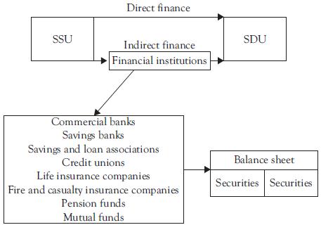
Figure 3.2 Financial flows
Direct finance occurs, for example, when a household or a business purchases a U.S. Treasury-bill at the weekly T-bill auction. In this case, the U.S. government is a savings-deficit unit. It is issuing Treasury-bills to finance its deficit spending.
Households and businesses purchasing T-bills are savings-surplus units (so long as they are net suppliers of funds to financial markets). They are purchasing the new government debt. Because the weekly auctions of Treasury bills occur at Federal Reserve Banks, these Reserve Banks are performing a brokerage function.
A second example involves household purchases of bonds newly issued by a utility company. It is direct finance because these households are directly purchasing securities issued by a savings-deficit unit (the utility company). Again, households making such purchases are classified as savings-surplus units if they are net suppliers of funds to financial markets.
Financial flows are described as indirect finance if there is financial intermediation. Intermediation occurs when funds pass through financial institutions.
What distinguishes these institutions from other businesses is that securities dominate both sides of their balance sheet. They issue securities, which appear on the right-hand (or liability) side of their balance sheet. Funds obtained from selling these securities are then employed to purchase securities for the left-hand (or asset) side of their balance sheet.
If financial institutions are to operate with a profit, they must have a positive spread. The spread is the difference between two balance-sheet rates. It is the average rate that a financial institution earns on the securities they own (from the left-hand side of the balance sheet) minus the average rate that pay on debt securities that they issue (from the right-hand side of their balance sheet). For example, if the average return on a bank’s assets is 5% and the average cost of its liabilities is 4%, the spread is 1%. The spread must be positive for a financial institution to be viable.
This raises an interesting issue. For a financial institution to operate successfully, it is apparent from Figure 3.2 that it must intercept the flow of funds from savings-surplus units to savings-deficit units. To operate with a positive spread, however, the financial institution must offer savings-surplus units a lower rate (on average) than they would obtain if they opted, instead, to purchase securities directly from savings-deficit units. The question, then, is: why would savings-surplus units agree to this arrangement?
The answer to this question provides insight into the operations of financial intermediaries. To induce savings-surplus units to purchase their securities with a lower average return, financial institutions must design financial instruments with distinct features that make them attractive to market participants. Investors must view these features favorably enough to cause them to purchase the securities even though they offer a lower average return. The growth and proliferation of financial institutions during the post-World War II period is testimony to their ability to accomplish this task.
The innovative features in the instruments offered by financial institutions are varied. Some instruments provide customers with favorable denominations. This is particularly true of depository institutions, where customers are able to deposit sums that vary anywhere from a few dollars to millions of dollars. Liquidity, too, is also an important feature, and depository institutions also offer instruments that are used as exchange media.
Many of the instruments offered by financial institutions allow owners to reduce their risk exposure. Deposits offered by banking institutions, for example, frequently carry insurance against default risk. Investment companies (or mutual funds) permit share owners to participate in the returns on a broadly diversified portfolio of securities. Life insurance companies insure against an untimely death by offering securities with death benefits.
Intertemporal Production and Exchange
The interest rate falls within the realm of intertemporal economics, or what Austrian theorist Eugen von Böhm-Bawerk called the “the present and future in economic life.”3 While the interest rate is not defined by everyone in the same way, it is useful to observe that the interest rate is intimately related to three intertemporal economic relationships: (1) the marginal productivity of capital; (2) the price of credit; and, (3) the marginal rate of time preference. Each of these phenomena has been employed in formulating a definition of the rate of interest. Understanding how these intertemporal phenomena are related to one another is central to the problem of defining the interest rate.
Marginal Productivity of Capital
Unlike land and labor, capital goods are the produced means of production. Moreover, they are produced for good reason. The production and use of capital goods, while necessarily more time-consuming (or “roundabout” according to Böhm-Bawerk), generally is productive. That is, the use of previously produced goods to produce additional goods generally results a net increase in the quantity of these goods. This net product, at the margin, is called the marginal productivity of capital (MPK).
The productivity of capital goods raises the issue of how to describe this net product that results from their usage. Böhm-Bawerk referred to it as interest or, more specifically, originary interest. Interest in this sense is the payment to the input capital. Unless it is placed in the context of the intertemporal valuation of goods, however, this payment is likely to vanish (or go to zero). If individuals make no distinction (or are indifferent) between an equal quantity of goods now or goods in the future, they will tend to accumulate capital goods currently until the marginal product of capital is zero. At that point, capital accumulation ceases and the interest rate is zero.
Price of Credit
Individuals can give up their claims on current goods to others, and receive in exchange claims on future goods. Contracts specifying such exchanges are loan contracts, or bonds. The excess of future goods (if any) resulting from this intertemporal exchange is also commonly called interest (or the interest rate when expressed in proportionate terms).4
Borrowers who issue these bonds are renting the use of money for a specified period of time. Thus, when used in this context, the interest rate is a rental payment for the use of borrowed funds. This rate is frequently described, alternatively, as the price of credit.
The price of credit, likewise, will tend to vanish unless it is placed in the context of the intertemporal valuation of goods. If individuals make no distinction (or are indifferent) between an equal quantity of goods now or goods in the future, they will readily exchange present and future goods with one another on equal terms. The price of credit in this case is zero.5
Marginal Rate of Time Preference
The phenomenon that keeps the marginal productivity of capital and the price of credit from potentially going to zero is time preferences. These subjective preferences represent how individuals value goods now relative to goods in the future, or present consumption relative to future consumption.
The marginal rate of time preference (MRTP) is a quantitative expression of these valuations for incremental units. It is the quantity of future goods an individual is willing to sacrifice for a specified quantity of present goods of comparable quality. It is normally formulated in proportionate terms, as in equation 3.10. If MRTP = 5%, for example, an individual is indifferent between a given quantity of present goods and 5% more future goods.
![]()
where dC1 and dC0 are changes in future goods (or consumption) and present goods, respectively. The ratio of these changes is an absolute value.
An individual who prefers present goods over future goods is said to have positive time preferences, i.e., MRTP > 0. One who is indifferent has neutral time preferences (MRTP = 0), and one who prefers future goods over present goods, negative time preferences (MRTP < 0).
Individuals are generally viewed as having positive time references. If that is the case, then the marginal productivity of capital and the price of credit need not vanish. The case of a positive price for credit (or interest) is considered below in the discussion of the real interest rate. The case for a positive marginal productivity of capital is discussed presently.
In the absence of a credit (and/or equity) market, all capital formation is internally financed. That is, all capital goods are financed through the saving of the economic unit accumulating capital goods. Each unit must weigh the value of current goods sacrificed against the value of the additional future goods resulting from the employment of those capital goods. With positive time preferences, the unit will accumulate capital goods (currently) up to the point where the marginal productivity of capital is equal to the marginal rate of time preference.
![]()
If the marginal productivity of capital were to exceed the marginal rate of time preference (MPK > MRTP), the individual will choose to further abstain from present consumption and accumulate more capital goods. Assume for example that the MPK is 6% and the MRTP is 5%. This individual would be indifferent between a given quantity of present goods and 5% more future goods. However, abstaining from present goods and accumulating capital goods results in 6% more future goods. The individual is clearly better off accumulating more capital goods, and will continue to do so until the equality in equation 3.11 is obtained. By similar reasoning, the individual will accumulate fewer capital goods whenever the marginal productivity of capital is less than the marginal rate of time preference, again until 3.11 is obtained. It is important to note that, in both cases, the marginal productivity of capital conforms to the positive rate of time preferences.
Defining Interest
While there is general agreement concerning the intertemporal nature of interest, there is no such general agreement about the definition of the interest rate. It has been defined as the return to the input capital and, alternatively, as the price of credit. Ludwig von Mises defined it yet another way: as the rate of time preference.6
There is good reason for defining interest in the manner of von Mises. It was noted above that both the return to capital and the price of credit tend to vanish (or go to zero) in the absence of positive time preferences. That is, both of these phenomena rest on the pillars of time preference. Moreover, both are simply different manifestations of how individuals are willing to exchange future goods for present goods.
For those reasons, defining interest as the rate of time preference is preferred. This expression is general enough to encompass different forms of intertemporal exchange such as credit transactions and the return to capital. As discussed below, this definition of interest can also be modified to accommodate the possibility of contract default in intertemporal exchanges.
In conventional parlance, however, the interest rate is most often discussed not as the rate of time preference, but as the price of credit. This is true in the world of finance, and particularly in discussions of money and monetary policy. While less preferred for the reasons just noted, on grounds of expediency that expression for interest is subsequently employed.
Interest Rates
The Real Interest Rate
The interest rate can be expressed either in nominal or real terms. The nominal (or money) interest rate is the price of credit expressed in terms of money. The real interest rate, sometimes referred to as the “pure” rate of interest, is the price of credit expressed in terms of physical units (or goods and services).
When markets are free, borrowers and lenders determine the price of credit. It is anticipated that these economic agents will act rationally, that is, that they will think in real terms. (Those who do not are said to suffer from “money illusion.”) It follows that, for such rational decision-makers, it is the real interest rate that influences their choices.
This makes the analysis of credit markets somewhat subtle, because the real interest rate generally is not observable. What we typically observe is the nominal rate of interest. The nominal rate is the one typically quoted in the financial media, and generally it is the rate explicitly negotiated in credit contracts. This means that economic agents think in real terms, but most often negotiate credit contracts in nominal terms.
The Positive Real Rate of Interest
With few exceptions, those who attempt to estimate the real interest rate obtain a positive number. A fundamental analytical issue, then, is explaining this empirical outcome—that the real rate of interest is positive. The theory advanced to account for this phenomenon is the existence of positive time preferences for consumption. As noted above, time preferences are concerned with how individuals value goods now relative to an equivalent amount of goods in the future (or present consumption relative to future consumption). An individual who prefers present consumption to future consumption is said to have positive time preferences. By contrast, one who is indifferent has neutral time preferences; one who prefers future consumption, negative time preferences.
If sufficient number of individuals have zero time preferences, the real interest rate will be zero. Those who wish to borrow in the credit market are able to obtain additional claims on current goods from lenders with zero time preferences. These lenders are indifferent between current consumption and future consumption, and willingly give up their claims to current goods in exchange for claims to an equal quantity of future goods. That is, they do so at a zero interest rate. Compensation in the form of a positive real interest rate is unnecessary because of their indifference between present and future consumption.
This is shown graphically in Figure 3.3. The supply curve for loanable funds follows the quantity axis. No matter what the demand for loanable funds, the real interest rate remains zero. Graphically, as the demand for loanable funds shifts from D0 to D1 to D2, the supply of loanable funds is perfectly elastic at the zero rate of interest.

Figure 3.3 Market for loanable funds
On the other hand, if a significant number of individuals have positive time preferences, the real interest rate will be positive. Now, individuals borrowing (in the credit market) to acquire more current goods must pay a positive real interest rate. The reason is that lenders with positive time preferences will not give up their claims on current goods unless they are compensated.
It is in this way that positive time preferences account for the existence of a positive real interest rate. Moreover, this real rate is a precise expression of those time preferences. Hence, the real interest rate is referred to as the rate of time preference. A 5% real interest rate, for example, indicates that individuals are willing to sacrifice present consumption if they are compensated by 5% additional future consumption.
Level of the Real Interest Rate
A graph of the loanable funds market is presented in Figure 3.4. Both sides of the market reflect the time preferences of market participants. The supply curve is a locus of points showing the willingness of economic agents to forego present consumption at different interest rates. A higher real interest rate represents a larger compensation for deferring present consumption. Consequently, more funds are supplied at higher real interest rates.
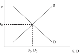
Figure 3.4 Market for loanable funds
The demand side of the market for loanable funds also reflects time preferences. Borrowers in this market obtain claims for present consumption from lenders. Some borrowers may be consumers desirous of consuming in excess of their income, i.e., dissaving. Others may be businesses wanting to finance the acquisition of additional capital goods by borrowing.
Borrowers must sacrifice future consumption in order to obtain claims for present consumption. The amount of the sacrifice is specified by the real rate of interest, which indicates the rate of exchange of future consumption for present consumption. With a smaller sacrifice (i.e., the lower the real interest rate), more funds are demanded by borrowers.
Price plays an allocative role in this market. The real interest rate allocates available funds among alternative users. At the equilibrium interest rate, r0, the quantity of loanable funds demanded is equal to the quantity supplied. The disparate plans of all market participants are rendered consistent with one another. It is adjustments in the real interest rate that brings about this consistency of plans.
When the plans of all economic agents are consistent with one another (at interest rate r0), resources in the economy are allocated in such a manner that aggregate saving is equal to aggregate investment (S = I). All resources released by those abstaining from present consumption are absorbed in the production of capital goods. These capital goods, in turn, are available for the future production of consumables.
As an expression of time preferences, the real interest rate is the market assessment of how economic agents are willing to exchange present and future consumption. When these time preferences change, so, too, does the real interest rate. Assume, for example, that there are reduced time preferences for present consumption. This can take several forms. Some individuals with positive saving may choose to save more. The result is a rightward shift in the supply curve of loanable funds (from S0 to S1 in Figure 3.5, left panel).

Figure 3.5 Market for loanable funds
Another possibility is that individuals previously dissaving choose to dissave less. In this case, the demand for loanable funds decreases and the demand curve shifts to the left (from D0 to D1 in the left panel). A third possibility is that there is a combination of the two. That is what is depicted in Figure 3.5, left panel. The supply of loanable funds increases and the demand decreases. At the previously prevailing interest rate (r0), there is now an excess supply of loanable funds. Competition among suppliers results in a decline in the equilibrium real interest rate. The new market clearing rate is r1.
Changes in the perceived marginal productivity of capital also cause time preferences to change. An increase in the productivity of capital, for example, increases business demand for capital goods. Capital goods are present goods, and this constitutes an increase in time preferences for current goods. The result is an increase in the demand for loanable funds. In Figure 3.5, right panel, the demand curve for loanble funds shifts to the right (from D0 to D1). At the previously-prevailing real interest rate, r0, there is now excess demand for loanable funds. Competition among those seeking claims to current consumption forces the real interest rate upward. The market clears at interest rate r1.
Risk and the Real Rate of Interest
Analysis of the real interest rate to this point has neglected risk factors.7 The “pure” interest rate was a risk-free rate. The introduction of risk can affect the level of the real interest rate because risk-averse lenders must be compensated for the risk that they incur as suppliers of funds to financial markets.
There are several types of potential risk that are of importance to market participants. Two are default risk and price risk. Default risk is the risk that the borrower will not repay funds that are advanced by lenders. If that occurs, the lender incurs financial loss. Given this possibility, borrowers generally must compensate lenders by offering a risk premium in the real rate.
Price risk, on the other hand, is the risk that the price of a debt security will vary during the holding period. It has significance to investors because they often do not know with certainty when the security will be liquidated. Selling a security whose price has fallen substantially results in a sizable capital loss. As a consequence, this type of risk, too, can give rise to a risk premium in the real interest rate.
The size of the risk premium, if any, in the real interest rate is dependent upon the risk preferences of market participants. For those who are risk-averse, less risk is preferred to more risk. If investors generally exhibit such preferences, the real rate will include a risk premium that embodies the market valuation of the risk involved.8 Greater risk is associated with a higher risk premium (and a higher real interest rate); less risk, with a lower risk premium (and a lower real rate).
Although we are unable to directly observe the preferences of market participants, rate patterns in the marketplace generally are consistent with risk-averse behavior as described above. The dominance of this type of behavior has significance beyond affecting the level of the real interest rate. With risk-averse behavior, the real interest rate no longer represents the rate of time preference for both borrowers and lenders. There is now a wedge between their time preferences in the amount of the risk premium.
This situation is graphically shown in Figure 3.6, where the loanable funds market in the presence of risk is compared to the same market when there is no risk. Consider, initially, the case with no risk. The supply and demand for loanable funds are represented by curves S and D, respectively. With price playing its customary rationing role, the loanable funds market clears at interest rate r1. This real interest rate represents the time preferences of both lenders and borrowers. At this rate, the quantity demanded of loanable funds (D1) is equal to the quantity supplied (S1).
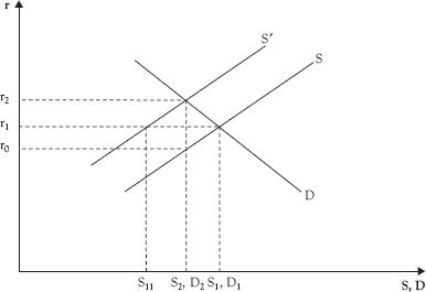
Figure 3.6 Market for loanable funds
Once risk is introduced, risk-averse lenders will require compensation for the risk they incur. Compensation occurs because they are less willing to lend than they were before. This is manifested in a leftward shift in the supply curve for loanable funds (from S to S′). For each quantity of loanable funds supplied, the real interest rate is now higher. At the previous equilibrium interest rate (r1), there is now an excess demand for loanable funds (D1 − S11). Competition among borrowers drives the real rate higher to its new equilibrium level, r2. The quantities of loanable funds supplied and demanded are now S2 and D2.
This new equilibrium interest rate (r2) is an expression of the time preferences of borrowers. It represents how much future consumption they are willing to sacrifice in order to consume more currently. r2, however, does not represent the time preferences of lenders. Instead, it represents the summation of the time preferences of lenders (r0) and the necessary risk premium (r2 − r0) given their risk-averse behavior.
In the absence of risk, lenders will supply a lower quantity of funds, S2, at rate r0 (a movement down supply curve S) than they would at r1. The rate r0 now represents their tradeoff of present and future consumption, or their time preferences. In the presence of risk, a risk premium (r2 − r0) is added to their rate of time preference, and lenders supply the same quantity of funds, S2, at the higher real rate r2. The risk premium now constitutes a wedge between the time preferences of borrowers and lenders.
The Nominal Interest Rate
The nominal interest rate is the price of credit expressed in monetary units. Most interest rate quotes are nominal rates. Three features of those nominal rates are discussed below. First, the nominal interest rate is related to bond prices. Second, the nominal interest rate is affected by inflationary expectations. Finally, the characteristics of bonds vary. As a consequence, there is not a single nominal rate, but rather an entire vector of nominal interest rates.
Bond Prices and Interest Rates
Bonds traded in financial markets represent borrowed funds. They are issued by borrowers and purchased by lenders. Associated with each bond is a price and an interest rate. Bond prices are an expression of the subjective value of the bonds to traders in the market. These valuations change and, as a consequence, so do bond prices.
Those issuing bonds usually are renting the use of money for a specified period of time. The rental payment for these funds is the interest rate, or the price of credit. Having stated this, it is important to state what the interest rate is not. The interest rate is not the price of money, as is sometimes claimed. The price of money, as noted above, is its exchange value relative to other things. Assuming that P is the average price of other things, then the purchasing power of money (or the price of money) is the reciprocal of P (see pp. 7−8 above).
Many bonds are actively traded in the secondary (or resale) market. In the secondary market, bond prices and nominal (or money) interest rates are inversely related. This occurs because the nominal interest rate for newly issued (or primary) debt constantly changes. Market traders respond to variations in the interest rate by revaluing previously issued bonds. This revaluation is necessary for previously issued debt securities to remain price-competitive with the newly issued debt.
An example of this kind of revaluation is presented in Exhibit 3.1. The bond traded is a perpetuity, i.e., it has no maturation date. The borrower issues the bond in Period 1 with a price of $1,000. The coupon payment of $50 is sufficient to induce lenders to purchase the bond. With this coupon payment, the bond owners receive 5 percent nominal interest on this investment.

Exhibit 3.1 Bond Prices and Interest Rates
In Period 2, market conditions change. The nominal interest rate on newly issued debt increases to 10%. The individuals who purchased perpetuities in period 1 continue to receive an annual interest (or coupon) payment of $50. If they choose to sell their bonds in Period 2, however, they will have to do so at a lower price. No one will pay them the $ 1,000 they initially paid for the bonds. At that price, those purchasing these perpetuities would only receive an interest rate of 5%. This is below the 10% rate they would receive when purchasing newly issued debt securities.
However, investors would be willing to purchase these perpetuities on the secondary market at a lower price. At a price of $500, the interest rate they would receive when purchasing these securities on the secondary market is equal to the 10% return on newly issued bonds. That is, $50/$500 = 10%. Thus, the price of the perpetuities falls to $500.
This example was for an increase in the nominal interest rate. If the nominal rate were to fall, the opposite occurs. Bond prices increase. In general, when the nominal interest rate changes in financial markets, prices of previously issued bonds in those markets move in the opposite direction.
Inflationary Expectations
The study of the relationship between the nominal and real interest rates draws upon the work of Irving Fisher. It is possible for these two rates to be the same. That is not the case, however, in an inflationary environment. Because the world of fiat money is a world of inflation, Fisher’s analysis of how bond traders adjust bond prices and interest rates in response to changes in inflation has assumed much greater importance.
Equation 3.12 below is known as the Fisher equation. It shows the relationship between nominal and real rates of interest, and how they are affected by inflation.
![]()
where i is the nominal interest,
r is the real interest rate, and
(dP/P)* is the expected rate of change of the average price during the term of the credit contract.
Credit contracts are ex ante relationships. Any inflation that occurs during the term of the contract will erode the purchasing power of the money loaned. Borrowers will repay lenders in monetary units that have less purchasing power than the money they borrowed. This affects the real wealth of both borrowers and lenders. As a consequence, rational economic agents (on both sides of the contract) must take inflation into account when entering credit contracts.
When credit contracts are consummated, the actual rate of inflation during the term of a contract is not known. What affects contracts, then, are the inflationary expectations of borrowers and lenders. According to Fisher, the expected rate of inflation [dP/P)*] is fully incorporated into terms of credit contracts—in the form of a higher nominal rate of interest. This is how the borrower compensates the lender for expected changes in the purchasing power of the money during the term of the contract.
This compensation appears as the last term in the Fisher equation [dP/P)*]. It is known as the inflation premium in the credit contract. Note that when expected inflation goes up, so too, does the nominal rate of interest. When inflationary expectations decline, the nominal rate falls commensurately.
These adjustments in the level of the nominal rate of interest are a market phenomenon. It is the way that borrowers and lenders respond to changes in the inflationary environment. When inflation increases, the purchasing power of the money loaned depreciates more rapidly. Lenders would like additional compensation in the form of a higher interest rate.
A higher interest rate, however, is not in the self-interest of borrowers. What motivates them to offer a higher rate is the competition for available funds in credit markets. With higher inflation, many assets are increasing in value. The price of farm land, for example, may rise from $2,500 per acre to $3,000 and then $4,000 per acre. Owners of assets that are appreciating in value are willing to bid up the price of credit because the assets they are purchasing with borrowed money are gaining in value.
An example of how participants in credit markets adapt to different inflationary environments is presented in Exhibit 3.2. In Case I, market participants expect price stability. As a consequence, the nominal and real rates are the same (3%). Assume individual A lends $100 to individual B for one year. At the end of the contract period, B pays A, $103. The payment consists of $100 in principal and $3 in interest. If inflationary expectations were correct, the $100 in principal will purchase the same quantity of goods at both the beginning and end of the contract period. Moreover, the $103 received by A will purchase 3% more goods and services than the $100 loaned. Thus, not only is the nominal rate of interest 3%, but the real rate is 3% as well.
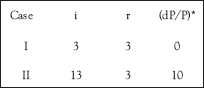
Exhibit 3.2 The Fisher equation
The world changes, and inflation increases. This affects expectations. In Case II, borrowers and lenders now anticipate 10% annual inflation. These higher inflationary expectations are incorporated into the terms of credit contracts. The nominal rate of interest increases from 3% to 13%. The difference, of course, is the higher inflation premium.
Now individual A loans individual B $100. One year later, B repays the loan with interest, or $113. Assuming expectations are correct, the $100 in principal returned will purchase 10% fewer goods and services than when the loan was made. The inflation premium of 10%, however, compensates the lender for this erosion in the purchasing power of the principal. That is, $10 of the $13 in nominal interest represents this compensation to the lender. $110 (of the $113) received by the lender will now purchase the same quantity of goods and services as the $100 initially loaned. What remains is $3 in interest. That $3 is the real interest rate in this example. The $113 received by the lender will purchase 3% more goods and services than the $100 initially loaned in this contract.
This market adjustment is shown graphically in Figure 3.7. In the market for loanable funds, the vertical axis is the nominal interest rate; the horizontal axis, the quantity of loanable funds. Initial equilibrium occurs at the nominal interest rate iI (or 3%). This corresponds to Case I in Exhibit 3.2. With expectations of zero inflation, the real rate of interest is also 3%.

Figure 3.7 Market for loanable funds
In Case II, inflationary expectations increase to 10%. Each nominal interest rate on the vertical axis now corresponds to a lower real interest rate. For example, the 3% nominal rate now corresponds to a real interest rate of negative 7% (versus a plus 3% before). As a consequence, lenders will want to lend less at each nominal interest rate. Borrowers will want to borrow more at each nominal rate.
These changes appear graphically as a leftward shift in the supply curve (from SI to SII), and a rightward shift in the demand curve (from DI to DII). The previously prevailing equilibrium rate of interest rate (3%) no longer clears the credit market. There is excess demand at this rate. Competition among borrowers for available funds causes the nominal rate of interest to move higher. At the 13% nominal rate, the credit market again clears. This nominal rate now corresponds to a 3% real interest rate. The market for loanable funds clears at the same real rate as before.
Fisher’s analysis, then, shows how open credit markets accommodate inflation. Although there are numerous empirical studies of Fisher’s theory, two observations are cited here to demonstrate how the theory often conforms to the data. First, the U.S mortgage rate recently fell below 4%. This is much lower than the rate in the early 1980s, which was nearly 17%. What would account for such a dramatic fall in the nominal rate of interest? Fisher’s analysis would suggest that the inflation rate in the early 1980s must have been considerably higher. Indeed, it was. The consumer price index (CPI) rose by 13.5% in 1980; in 2012, only 2.1%.
A second observation is that nominal interest rates vary substantially across countries. Based on Fisher’s analysis, countries with relatively low inflation should have relatively low nominal rates of interest. Alternatively, relatively high inflation countries should have correspondingly higher nominal rates of interest. That, too, generally is the case.
A final issue addressed here has to do with forecasting errors. In the previous examples, it was assumed that expectations were correct, that is, there were no forecasting errors. In those cases, (dP/P)* = dP/P. Expected inflation is equal to actual inflation or, alternatively, ex ante inflation is equal to ex post inflation.
Most often, there are forecasting errors. Such errors are important because they result in transfers of wealth. The nature of the transfer depends on whether market participants forecast the inflation rate too high or too low. When they forecast it too high [(dP/P)* > dP/P], wealth is transferred from borrowers to lenders. When (dP/P)* < dP/P, the opposite occurs. Wealth is transferred from lenders to borrowers.
Examples of both types of transfer are presented in Exhibit 3.3. Case I is the credit contract. It is an ex ante relationship, with a nominal interest rate of 8%. The expected rate of inflation during the term of the contract is 5%. Given these expectations, the anticipated real rate of interest is 3%.

Cases II and III are two different ex post scenarios. In Case II, the actual rate of inflation during the term of the contract was 10%. This was higher than expected [(dP/P)* < dP/P]. Market participants anticipated a real interest rate of 3%, but the actual (ex post) real rate was a negative 2%. This unexpected lower real rate benefited borrowers at the expense of lenders. Had lenders known that the real interest rate was going to be negative 2%, they never would have entered the contract. Had borrowers known, they would have borrowed much more.
This forecasting error transferred wealth across the credit contract from lenders to borrowers. The form of the transfer was the lower real interest rate. Enormous amounts of wealth have been transferred in this way.
A recent historical example occurred in the United States in the 1970s and early 1980s. Inflation accelerated sharply. As a consequence, actual inflation rates rose above anticipated rates of inflation. While borrowers were feeling very good about long-term loan contracts consummated in the 1960s, lenders were not. Indeed, this forecasting error caused many lenders to declare bankruptcy. Among them were numerous banks and savings and loan associations. So severe was the problem that the U.S. government deemed it politically desirable to funnel large quantities of tax dollars into failing financial institutions.
In Case III, the actual rate of inflation (0%) is lower than expected inflation. This situation benefits lenders (at the expense of borrowers). The ex ante real interest rate was 3%. The ex post real rate was 8%. Many borrowers would have refused to enter credit contracts had they known the real interest rate was going to be this high.
The wealth transfer, in this case, is from borrowers to lenders. It is in the form of a higher than expected real rate of interest. The United States experienced this situation in the 1980s, when the rate of inflation decelerated sharply. Many borrowers declared bankruptcy. This included farmers, agricultural equipment dealers, and building contractors.
Farmers who borrowed to acquire more land expected that land values would appreciate (as they had when inflation accelerated in the 1970s). They anticipated repaying the loans by selling commodities at higher prices (again, like the 1970s). These events did not come to pass.
A similar fate befell building contractors. Many borrowed to construct houses prior to selling them. This market tactic had “worked” for much of the 1970s. When the anticipated rise in housing prices did not materialize, expected profits turned to losses.
In a very general sense, Fisher’s interest-rate model is yet another testimony to the resiliency of markets. Through nuances in prices, markets transmit all kinds of information. In this case, the information transmitted in bond markets is the expected rate of inflation. This analysis has been especially useful in our contemporary world of fiat money, where inflation rates largely have been positive and often quite volatile. In those cases where governments have not arbitrarily fixed interest rates, Fisher’s analysis shows the adaptation that occurs in financial markets in response to the vagaries of inflation.
The Vector of Nominal Interest Rates
Hitherto, the discussion has focused on a single interest rate—the rate of interest. That simplification facilitated discussion of the market for debt securities. In reality, there are many different interest rates. This is reflected in the interest rate vector in 3.13, where there are n different nominal interest rates. Individual rates in this vector might represent the interest rate on federal funds, 3-month Treasury bills, 6-month Treasury bills, 10-year Treasury bonds, corporate bonds, mortgages, 6-month certificates of deposit, and rates on numerous other debt securities.
![]()
Debt securities have different interest rates because they are not identical, i.e., they have different characteristics. Interest-rate differentials such as those in 3.13 reflect market pricing of these characteristics. Many of these characteristics were discussed earlier in the chapter. One example is inflationary expectations and their impact on nominal interest rates. Expected inflation for the next six months may differ from expected inflation for the next two years. Both of these may differ from expected inflation for the next 10 years. Because debt securities vary by maturity, the inflation premium will not be the same for securities of different maturity. This may account for a portion of the interest rate differences in equation 3.13.
Interest rates in vector 3.13 may also vary because securities do not all have the same risk characteristics. Nuances in risk are priced into securities by market participants. An example is default risk, which can vary considerably across loan contracts. Differences in default risk may reflect the fact that individual borrowers face different financial environments. Borrowers may also warrant different rates if they have different ethical standards regarding the repayment of debt.
A case where default risk is considered relatively low is debt securities issued by the U.S. government. Like other national governments, the U.S. government has an advantage over other borrowers because it has the power to both tax and print money. Moreover, the U.S. government has a record of not defaulting on its credit contracts. As a result of these factors, market participants generally consider it very unlikely that the U.S. government will default on its debt obligations. That makes it possible for the U.S. government to borrow at relatively low nominal interest rates. By contrast, most other borrowers pay higher rates. At the other end of the risk spectrum from U.S. government securities are pay-day loans and loans at pawn shops. Default risk and interest rates are much higher for these securities.
Other factors that occasion variations in nominal interest rates include tax features and time preferences. Intergovernmental relations result in some securities having a more favorable tax status. Interest on state and local government securities, for example, generally is exempt from federal income taxes. Interest on U.S. government securities, in turn, is exempt from state income taxes. Because investors are interested in after-tax income, such differences in tax treatments are incorporated into bond prices and rates.
Time preferences have an impact because it is unlikely that the willingness of individuals to trade-off current consumption for consumption one year from now is the same as their willingness to trade-off current consumption for consumption five years, ten years, or twenty years from now. If that is the case, differences in time preferences will also account for some of the interest-rate variations observed in equation 3.13.
The Term Structure of Interest Rates
Not only do interest rates differ at a given point in time, but returns on securities can vary based on differences in their maturity. A curve showing the yields of a set of securities differing only in maturity is known as the term structure of interest rates, or the yield curve. Each point on the curve is an ordered pair, and associates the maturity of a security with its yield. While it is not easy to find actual situations where securities differ only in their maturity, a popular rendition is to show the different yields on securities issued by the U.S. Treasury.
Analysis of the term structure of interest rates is related to explaining its shape. Three yield curves with differing shapes are presented in Figure 3.8. The yield curve in Panel (a) is horizontal. With a horizontal yield curve, security yields do not vary by maturity. The yield on a six-month security is the same as the yield on one-year, two-year, three-year, and ten-year securities.
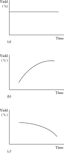
Figure 3.8 The term structures of interest rates.
The yield curve in Panel (b) is ascending. With an ascending yield curve, the yield increases with the time to maturity. Hence, the yield on a six-month security is less than the yield on a one-year security which, in turn, is lower than the yield on a two-year security. From an empirical standpoint, the yield curve most often assumes this form. Consequently, the ascending yield curve is sometimes referred to as the normal yield curve.
The term structure depicted in Panel (c) occurs much less frequently. Referred to as a descending yield curve, it is more likely to happen when inflation is relatively high.
For a descending yield curve, the yield on a six-month security is higher than the yield on a one-year security which, in turn, is higher than the yield on a two-year security. Yields on three-year, five-year, and ten-year securities are sequentially lower.9
Forward Rates
Implicit in any term structure of interest rates is a set of forward rates. These rates are not actual interest rates. Instead, they implied reinvestment rates. They are rates that would have to prevail if a sequence of investments in short-term securities is to have the same over all return as the return on a long-term security. The sum of the maturities for the short-term securities must equal the maturity of the long-term security.
Assume, for example, that bond A matures in one year and bond B matures in three years. The forward rate (in this case) is the interest rate on a two-year bond, available one year from now, that causes the compounded yield on the one-year bond (A) and two-year bond to equal to the compounded yield on the three-year bond (B). Thus, the proceeds from owning the one-year bond and investing the proceeds (at maturity) in the two-year bond are identical to the proceeds from owning the three-year bond. Equation 3.14 expresses this relationship symbolically.
![]()
where R3 is the current nominal (or spot) rate on a three-year bond,
tR1 is the current nominal rate on a one-year bond, and t+1r2 is the annual forward rate on a two-year security available one year from now.
Inserting numeric values, assume that the one year nominal rate is 4% (tR1 = 4%) and the three-year rate is 5% (tR3 = 5%). The implicit two-year forward rate in this case is 5.504%, i.e., t+1r2 = 5.504%.
Forward rates such as this one are strictly mathematical calculations. They assume importance, however, because they are given behavioral content in current explanations of the term structure of interest rates. Three alternative theories of the term structure are presented below.10
Unbiased Expectations Theory
This theory relies upon expectations to account for differences in yields for securities that differ only in their maturity.11 Each interest rate in a given term structure of interest rates is determined by expected future interest rates. Moreover, these expected future interest rates are operational. It is possible to compute them because forward rates have important informational content. According to the unbiased expectations theory, each forward rate implicit in the term structure is an unbiased estimate of the expected future interest rate for that same period.
With ρ representing the expected future interest rate, this relationship between forward rates and expected future interest rates is presented in equations 3.15 and 3.16. In 3.15, the forward rate for a j-year security available i years from now (t+irj) is equal to the expected interest rate on the j-year security available i years from now (t+iρj). The unbiased nature of the forward rate is exhibited by differencing the two rates, as in 3.16.
![]()
![]()
To further illustrate the relationship between forward rates and expected future interest rates, consider equation 3.17. Because all forward rates are of the form t+ir1, each is a one-year forward rate. According to the unbiased expectations theory, the forward rate on a one-year security available one year from now (t+1r1) is the estimate of the expected interest rate for a one-year security available one year from now (t+1ρ1). t+2r1, in turn, serves as the estimate of the expected interest rate on a one-year bond available two years from now (t+2ρ1). A similar interpretation is attached to the other forward rates. It follows that the long-term rate under consideration (tRn) is determined by this set of expected future interest rates.
![]()
where tRn is the current (or spot) interest rate on an n-year bond at time t, and
t+ir1 is the forward rate on a one-year bond at time t + i.
The cogency of this argument about the nature of forward rates is not contingent upon the fact that all forward rates in 3.17 are one-year rates. Forward rates could have any maturity less than or equal to n−1. What is germane about the argument, however, is that it generalizes to all nominal rates for a given term structure of interest rates. That is, each current interest rate on the yield curve is determined by expected future interest rates. That is the essence of the unbiased expectations theory.
The proposition that current interest rates are determined by expected future interest rates begs the question about determinants of expected future interest rates. While the unbiased expectations theory does not directly address this issue, one would anticipate that factors influencing expected future rates would not differ from those affecting the level of the current interest rate. If that is correct, then phenomena such as time preferences for consumption and expected inflation influence the shape of the yield curve. Default risk and money risk, however, largely do not. The reason is that the unbiased expectations theory generally presumes that the activities of bond traders squeeze risk premiums out of the term structure of interest rates.
There are three important implications of the unbiased expectations theory. First, expectations about future interest rates determine current interest rates. The current yield on a long-term bond is a geometric average of the current yield on a short-term bond and expected yields on a series of sequential short-term bonds whose maturities sum to the maturity of the long-term bond. In equation 3.17, for example, the long-term interest rate (tRn), is a geometric average of the one-year spot rate (tR1) and the expected interest rates for a sequence of n−1 separate one-year bonds. The maturities of these short-term bonds sum to n, the maturity of the long-term bond.
A second implication of the unbiased expectations theory is that the significance of maturity diminishes for the bond investor. If one considers an n-year investment period, the expected return is the same whether one purchases an n-year bond or a series of shorter term bonds and reinvests the proceeds. One such set of possibilities is presented in Figure 3.9. The compounded return with investment plan A is (1 + tRn)n. In this case, the investor purchases an n-year bond. For plan B, the investor purchases an n−1 year bond and invests the proceeds (at maturity) for one year. In plan C, the investor purchases an n−2 year bond and, at maturity, purchases sequentially two one-year bonds.

Figure 3.9 Returns on an n-year investment
In the final case, the investor purchases a sequential series of one-year bonds. With forward rates serving as unbiased estimates of expected future rates, the expected return for all n of these investment plans is the same. The maturity of the instruments selected has no bearing on the investor’s expected n-period return.
A final implication of the unbiased expectations theory is that it provides an explanation for variously shaped yield curves. For a horizontal yield curve [as in Figure 3.8, panel (a)], the level of the interest rate is not expected to change. With expected future rates the same as the current short-term rate, the average of these expected rates is identical to the current short-rate.
An ascending yield curve [Figure 3.8, panel (b)] implies that bond traders expect interest rates to rise in the future. That is necessary if the geometric average of these expected future rates is above the current short-term rate. One thing that could occasion such a pattern of expected future rates is inflationary expectations, e.g., if investors expected future inflation to be higher than current inflation.
Finally, descending yield curves, which are empirically rare, occur when investors expect interest rates to fall. This normally happens when interest rates are relatively high (by historical standards). In this situation, the expectation that rates would return to more normal levels would give rise to a negatively sloped yield curve.
One of the principal weaknesses of the unbiased expectations theory is that it assumes that transactions costs are unimportant. That is necessary if forward rates are to serve as unbiased expectations of expected future interest rates. For, if transactions costs are important, they constitute a portion of each forward rate. In this case, forward rates are higher than expected future interest rates. That is, they are (upward) biased estimates of expected future interest rates.
Liquidity Preference Theory
Diminution of the risks associated with bond ownership is a feature of the unbiased expectations theory. While subject to variation, both money risk and credit risk generally are viewed as positively related to the maturity of a debt instrument. This suggests that owning long-term bonds is riskier that owning short-term bonds. Given this “constitutional weakness” on the long side, the liquidity preferences of risk-averse investors will influence their portfolio selections. They will prefer to own shorter term securities unless they are compensated for the additional risk associated with owning long-term bonds. Such considerations form the basis of the liquidity preference theory of the term structure of interest rates.12
If risk-averse bond traders are compensated for assuming risk, bond interest rates will contain a risk premium. Forward rates no longer are unbiased estimates of expected future interest rates. The bias in forward rates, as shown in 3.18, is in the amount of the risk (or liquidity) premium. That is, the forward rate exceeds the expected future interest rate by the amount of the liquidity premium (t+iLj). Alternatively, the forward rate is equal to the expected future interest rate plus the risk premium.
![]()
where t+iLj is the liquidity (or risk) premium on a j-year bond available i years from now.
The bias in forward rates varies with the maturity of a debt instrument. Generally, the longer the maturity of an instrument, the higher is the risk premium. This reflects the notion that both default risk and money risk normally increase with the maturity of a debt instrument. If risk and maturity are strictly positively related, then the term structure of liquidity premiums is upward sloping. That is the case in 3.19.
![]()
The presence of a term structure of liquidity premiums imparts an upward bias to the term structure of interest rates. If for, example, the expected interest rate is anticipated to remain the same, the yield curve is ascending. This case is depicted in Figure 3.10 below.
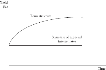
Figure 3.10 Term structure of interest rates.
The yield curve will also be ascending if future interest rates are expected to increase. In the case where expected interest rates are expected to fall, the shape of yield curve can be ascending, horizontal, or descending. It depends on the pattern of term structure of expected interest rates in relation to the term structure of liquidity premiums.
In the case of the descending yield curve, for example, the positive slope of the term structure of liquidity premiums is not of sufficient magnitude to offset a downward sloping term structure of expected interest rates.
The upward bias in the term structure under the liquidity preference theory is consistent with historical patterns in rates. From an empirical perspective, the yield curve most often is ascending, and is frequently referred to as the normal yield curve. Empirical dominance of the normal yield curve is precisely what one would expect under the liquidity preference theory of the term structure.
Market Segmentation Theory
The final theory of the term structure is the market segmentation theory. Markets for bonds of different maturity are segmented, and bonds of different maturity do not serve as substitutes for one another. The rationale for such market segmentation is the risk-averse behavior of market participants. In this case, however, the primary concern is with income risk, rather than money or default risk.
Income risk is the risk that relevant future income flows are subject to wide variation. One strategy for attempting to reduce this type of risk exposure is through the careful selection of bond maturities. Maturity selection, in this case, assumes the form of definite maturity preferences on the part of both individual borrowers and lenders.
Borrowers may reduce income risk by matching the maturity of their debt issue with their anticipated future cash flows. A corporation borrowing to finance a new plant, for example, may prefer to issue a long-term bond so that repayments coincide with the cash flow generated with its expanded production capacity.
Lenders, too, may have very specific maturity preferences. Households face income risk when accumulating assets in order to finance college education for their offspring. In order to reduce that risk, they may select debt instruments whose maturities are temporally aligned with dates of those anticipated college education expenses.
Financial institutions interested in reducing their income risk frequently do so through maturity matching. That is, they may attempt to match the maturity structure of their assets with the maturity of their liabilities. Banks, with a preponderance of short- and intermediate-term liabilities, may accomplish this by selecting short and intermediate-term assets for their portfolios. If interest rates subsequently increase, both revenues and costs rise. With rate decreases, revenues and costs fall commensurately.
In contrast to banks, life insurance companies have liabilities that are long-term and somewhat predictable. Maturity matching, in their case, involves the selection of longer-term bonds. These may include corporate bonds and mortgages.
Under the strict version of the market segmentation theory, borrowers and lenders have very specific maturity preferences, and are disinclined to deviate from those preferences. Bonds of different maturity are not substitutable for one another, and the term structure is determined by the supply and demand for securities at each level of maturity. Changes in supply or demand conditions for a particular level of maturity, in turn, result in a shift in the term structure of interest rates.
A different debt management policy by the Treasury, for example, will have an impact on the yield curve. The decision to issue a larger portion of the debt in the form of long-term bonds will increase long-term rates relative to short-term rates. Accordingly, the slope of the yield curve increases. Similarly, more long-term corporate borrowing is expected to increase long-term rates without spilling over into short term maturities.
A more moderate version of the segmented markets theory also has the term structure determined by specific maturity preferences on the part of both borrowers and lenders.13 With somewhat less rigid preferences, market participants may be enticed to deviate from their “preferred habitat” if the inducement is sufficient. If long-term rates rise significantly relative to short-term rates, banks and other depository institutions may choose to lengthen the maturity structure of their assets. This might occur even though the maturity structure of their liabilities remains unchanged. In the absence of sizable yield inducements, however, the expectation is that market participants will adhere to their preferred maturities.