
Monetary Policy in a World of Fiat Money
Most of man’s accumulated experience is with commodity money. Fiduciary money, by contrast, is relatively new. It has only been with us for the last several centuries. Like commodity money, the origin of fiduciary money generally is viewed as a spontaneous market development. The supposition is that the process that led to both of these types of money involved attempts by individual economic agents to reduce the transactions costs associated with voluntary exchange.
Nearly all money in use today is fiat money. As largely a 20th century phenomenon, this is a relatively new form of money. Unlike the other two types of money, the adoption of fiat money was not a spontaneous market development. It mainly came about through coercive acts of governments. Those undertaken by the U.S. government in 1933 are a case in point. President Roosevelt, acting on authority granted by Congress, issued an executive order making it illegal to hold monetary gold, with all outstanding monetary gold confiscated through forced exchanges.1 These actions effectively eliminated the convertibility option of the existing fiduciary money arrangement. Contracts relating to money ownership were not the only ones affected. All other contracts (such as bonds) written in terms of monetary gold were, likewise, summarily voided.
While individual economic agents generally preferred fiduciary money to fiat money, governments clearly did not.2 The convertibility option associated with fiduciary money significantly constrained government control over money. The reason was that excessive issue of fiduciary money threatened the integrity of the convertibility option, raising the specter of a financial panic. Elimination of the convertibility option removed that constraint, and gave individual governments the freedom to issue money at will.
With less than a century of continuous usage of fiat money, our relative lack of experience gives us a limited window for assessing the consequences of government control of money. One thing about fiat money, however, is abundantly clear. Under government control, changes in the quantity of money are not a random process. Decisions by governments across the world have led to unprecedented increases in the quantity of money.
Effects of Fiat Money
Despite our limited experience with fiat money, enough time has passed to permit a few tentative generalizations relating to its usage.
Monetary Nationalism
The adoption of fiat money accomplished its major objective. Governments now have much greater control over money. Instead of a global monetary system integrated by the use of a common money (or monies), we now have monetary nationalism. With a few exceptions, each country has its own money. Each of these monies is loosely linked to one another by activities in foreign exchange markets. Under this arrangement, individual countries are free to employ that particular monetary policy that best suits policymakers in the country. This was a major motive for moving away from fiduciary money. In this respect, then, the adoption of fiat money was a success.
Inflation
While national governments have much greater monetary autonomy in a world of fiat money, virtually all of them have used their monetary sovereignty in a similar manner. They have increased the quantity of fiat money. As a consequence, all countries share a common experience: inflation. The inflation has been continuous and, in many cases, pronounced. As a result, the period since the adoption of fiat money has appropriately been dubbed the age of inflation.
Data assembled by economic historians suggest that this title is well deserved. Rates of inflation that followed the adoption of fiat money are without precedent. David H. Fischer identifies four great inflations of the past millennium: the medieval inflation, the 16th century inflation, the 18th century inflation, and the 20th century inflation.3 Each of these inflations was widespread as evidenced by its impact on residents in many different countries. Inflation data for one of those countries, England, are presented in Table 5.1. Note that the rate of price increase during the inflation of the 20th century far exceeds that for any of the other three great inflations. Average annual fiat money inflation in England, 5.6%, was more than four times the average inflation rate for the 16th and 18th century inflations, and nearly 10 times the average inflation rate recorded during the great medieval inflation.
Table 5.1 Four Great Inflations in England (Average Annual Inflation Rate)
| I. Medieval Inflation (1265–1360) | 0.6 |
| II. 16th Century Inflation (1475–1650) | 1.3 |
| III. 18th Century Inflation (1730–1810) | 1.3 |
| IV. 20th Century Fiat Money Inflation (1931–2007) | 5.6 |
Sources: Phelps Brown and Hopkins (1956). Data for 1954–2007 are from International Financial Statistics: Yearbook, (various issues, International Monetary Fund).
The preeminence of the 20th century inflation, in terms of magnitude, is even more remarkable when one considers that fiat money was only widely adopted about one-third of the way through the century. As a consequence, most of the 20th century inflation accrued in the last half of the century. Average annual inflation in the United Kingdom, for example, was 6.5% from 1960–2002. Numerous other countries experienced double-digit average inflation for this period. This data leaves little doubt that the other three great inflations pale by comparison with 20th century inflation.
The effects of 20th century fiat money inflation on the purchasing power of money have been devastating. Table 5.2 shows the cumulative decline in the purchasing power of money in each of 55 countries for the 47 year period from 1960–2007. Note the breadth of the inflation experience. Massive depreciation in the exchange value of money occurred in all 55 countries. None fared better than Panama, where money lost more than 70% of its value. The median country on the list is Greece, where the exchange value of money declined by 98.8%. In 26 of the countries, money lost in excess of 99% of its purchasing power.
Table 5.2 Percent Depreciation in Value of Money: 1960–2007

Note: Data series for some countries begin after 1960. Starting dates for those countries are indicated by parentheses, e.g., Zimbabwe (65).
Source: International Financial Statistics: Yearbook (various issues, International Monetary Fund).
Reduced Services of Money
The plummeting exchange value of the world’s currencies has important implications for the services provided by money. Throughout the world, money has largely ceased to serve as a long-run store of value. This is manifested differently in various parts of the world. In the United States, individuals hold money balances almost exclusively for transactions purposes. Wealth accumulation occurs primarily via other assets such as stocks, bonds, and real assets.
In the less developed countries, on the other hand, one frequently observes a plethora of partially completed homes. The decision to build a home in stages, and over a period of years, is grounded in economic logic. Given the depreciation in the purchasing power of money in those countries, the poor of the world would never achieve home ownership through savings accumulated in the form of money balances.
In the more extreme cases of inflation, money often is rejected as a medium of exchange. The transactions costs associated with using the country’s money are deemed excessive. In rejecting the money of their own country, individuals sometimes select that of another country (such as U.S. dollars) for use as an exchange medium. This phenomenon is known as currency substitution. An alternative to currency substitution is reversion to barter. Even though the transactions costs associated with barter are often relatively high, in these cases, they are lower than when using money.
In responding to the monetary chaos they have created, governments often call in the old currency and replace it with a new currency. The rate of exchange can involve thousands of units of the old currency for one unit of the new. Because the old currency is discredited in a major way, it is common to give the new currency new colors and a new name. Once implemented, such monetary reform positions government to once again expand the quantity of fiat money at its own discretion.
Lower Economic Growth
Fiat money has been a vehicle for the transfer of massive quantities of resources from the private sector of the economy to government. This is especially true in many less developed countries, where money growth rates are relatively high. Historically, unpopular means such as taxation or other coercive measures have been the principal method for governments to increase their ownership of resources. The ability to print fiat money has given them an attractive alternative. By spending the money that they create, governments are able to wrest resources away from individuals without having recourse to more direct forms of coercion.
This additional source of finance has permitted 20th century governments to become much larger. A major consequence of the adoption of fiat money, then, is that it greatly enhanced the economic power of government relative to that of individuals. Given that more rapid economic growth generally is associated with greater individual economic freedom and more secure property rights, widespread use of fiat money has, no doubt, led to a reduction in world economic growth (relative to what it otherwise would have been). Because the alternative is a path not taken, it is difficult to know the magnitude of the reduction in living standards.
Expansion of Fiat Money: Motives
Our current age of inflation is a direct result of adopting fiat money. With inflation largely orchestrated by governments, the question of motivation arises. Is it in the self-interest of governments to expand the quantity of fiat money? The answer to this question is in the affirmative. Self-interested governments are driven by two principal motives.
One is seigniorage, or government revenue from money creation. Government control of money has permitted a significant reallocation of resources—from the private sector of the economy to government. Consequently, the world of fiat money is not only a world of inflation, but also one characterized by the rapid growth of government.
The second motive is found mainly among governments in several of the relatively industrial and market-oriented economies of the world. Influenced by the writings of British economist John Maynard Keynes, these governments have used monetary policy as a tool in the attempt to control movements in the aggregate economy. These efforts have resulted in significant money creation accompanied by inflation.
Seigniorge
The motive for most increases in the world money supply is seigniorage. Governments around the world consume vast quantities of resources. One way for them to wrest these resources from the private sector is taxation. As noted above, however, taxation generally is politically unpopular. Moreover, many governments of the world do not have fiscal systems in place that generate the quantity of tax revenues necessary to finance their desired expenditure programs. This is especially true in less developed countries, where greater use of currency in effectuating exchanges, more limited voluntary tax compliance, and the lack of legitimacy significantly hamper government’s quest for tax revenues.
An alternative to taxation is for government to finance expenditures by printing money. This can assume several forms. First, government can simply print new currency and spend it. There are numerous historical examples of this. One occurred during the Revolutionary War in this country, when the Continental Congress authorized the printing of currency (Continentals) to pay soldiers and to finance other wartime expenditures.
A second form is where the Treasury issues new bonds and places them directly with the central bank. In return, the Treasury receives an increase in its cash balance at the central bank. When the Treasury spends this additional cash balance, the quantity of money in circulation rises. This form of money creation is described as closed market operations in Chapter 4. It is popular throughout much of the world, and accounts for the bulk of fiat money creation.
A third, and more subtle form, is when the central bank monetizes debt issued by the Treasury. This is mainly possible in countries (such as the United States) that have encouraged the development of open financial markets. Monetizing debt occurs when the Treasury finances its expenditures by issuing bonds in the market. Those purchasing the newly issued bonds lose cash balances. The central bank replenishes this loss of private-sector cash balances through an open market purchase (equivalent in value to the Treasury bond sales). This joint Treasury/central bank venture results in additional Treasury cash balances at the central bank with no (net) loss of cash balances in the private sector. When the Treasury spends its new cash balances, the money supply increases.
The Seigniorage Tax
Printing money is posed as an alternative to taxation. It too, however, is a form of taxation. Unlike other taxes, though, it is a hidden or covert tax. The burden of this tax is borne by holders of (real) money balances. They are not presented with a tax bill but, instead, find that the additional inflation occasioned by government money creation adversely affects their money holdings. These cash balances now purchase fewer goods and services than they did before, i.e., their real cash balances have decreased.
The nominal seigniorage (S), in this case, is the money value of the goods and services that government is able to buy with the money it prints. Assuming that all money is government money, nominal seigniorage is equal to the increase in the money supply (dM, where dM > 0). Equation 5.1 shows the level of nominal seigniorage.
![]()
![]()
The quantity of goods and services (dM/P) the government can actually purchase with this new money is the real seigniorage, or s. In equation 5.2, real seigniorage is written as the product of the rate of growth of the money supply (dM/M) and the quantity of real money balances (M/P). This permits us to see more clearly the genesis of real seigniorage.
The total seigniorage tax on holders of real money balances is equal to the growth rate of money (dM/M) times the level of real money balances (M/P). To demonstrate this, recall Fisher’s quantity theory of money. A given growth rate for money increases the growth rate of prices by the same proportion. A 10% rate of money growth, for example, causes dP/P to be 10% higher than it otherwise would have been. Thus, real money balances depreciate by 10% more than they otherwise would, or by dM/M.
In equation 5.2, then, the growth rate of money is the tax rate that is applied to the quantity of real money balances, the tax base. The product of the two is the amount that real money balances fall as a consequence of money creation. This tax on holders of real money balances is precisely equal to the (real) government revenue from money creation, or s.
Maximum Seigniorage
The maximum amount of seigniorage government can collect is complicated by the fact that taxpayers are sensitive to tax rates. In this case, rational economic agents reduce their desired holdings of real money balances as inflation increases. That is, as the tax rate increases, the tax base declines. In equation 5.2, increases the growth rate of money (dM/M ↑) result in lower holdings of real money balances (M/P ↓).
Whether additional money creation increases real seigniorage depends on the relative strength of these two opposing forces. The tax rate elasticity of the tax base is the appropriate measure of this.
![]()
Table 5.3 shows the various possibilities. If η > −1, the numerator is smaller (in absolute terms) than the denominator. Hence, the tax base is changing less rapidly than the tax rate. In this case, increases in the growth rate of money result in higher real seigniorage.
Table 5.3 Money Growth and Seigniorage
| dM/M | s | |
| η > − 1 | ↑ | ↑ |
| η = − 1 | ↑ | → |
| η < − 1 | ↑ | ↓ |
If (in absolute terms) the tax base changes more, in proportionate terms, than does the tax rate, η < −1. This is the third case in Table 5.3. The increased sensitivity of taxpayers to tax rates means that a higher growth rate for money now results in less real seigniorage. A government desirous of more seigniorage must now reduce the growth rate of money.
It follows that a government interested in maximizing real seigniorage should increase the growth rate of money up to the point where η = − 1. At this point, the (proportionate) increase in the tax rate is exactly offset by the (proportionate) decline in the tax base. Further increases in the growth rate of money reduce real seigniorage. In Figure 5.1, maximum seigniorage occurs with tax rate (dM/M)2.
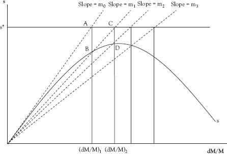
Figure 5.1 Seigniorage with hyperinflation
Hyperinflation
Inflation can degenerate into hyperinflation, or a very high rate of inflation. When this happens, inflation can reach hundreds or even thousands of percent per month. There have been numerous instances of hyperinflation, and all are associated with the use of fiat money. Without the constraint imposed by a convertibility option, governments are free to create massive quantities of money. Some have chosen to do so.
Data from some of the major 20th century episodes of hyperinflation are presented in Table 5.4. One of the most dramatic cases occurred in Hungary immediately after World War II. Inflation averaged 19,800% per month for nearly one year. To grasp the magnitude of this inflation, consider the impact on the price of a candy bar selling for $ 1. With this inflation rate, the price would increase to nearly 400 million dollars in two months.
Table 5.4 Episodes of Hyperinflation
| Country | Dates | Average inflation rate (per month) |
| Germany | Aug. 1992-Nov. 1923 | 322 |
| Greece | Nov. 1943-Nov. 1944 | 365 |
| Hungary | Aug. 1945-July 1946 | 19,800 |
| Poland | Jan. 1923-Jan. 1924 | 81 |
| Russia | Dec. 1921-Jan. 1924 | 57 |
Source: Cagan, Philip (1956).
Hyperinflation occurs when a government’s quest for seigniorage becomes dynamically unstable. Government prints more money in order to spend more. But, the ensuing inflation means that government is actually able to purchase fewer goods and services than before. Therefore, the government prints even more money. This results in even higher inflation, again reducing the purchasing power of the money created by government. Additional money is created, and the acceleration of money growth eventually spirals out of control.
The massive quantities of money created by government put enormous upward pressure on the right-hand side of Fisher’s equation of exchange. Huge increases in M are dissipated in the form of a rapid rise in P. But, a second factor is exacerbating the impact on P. The rapid increase in prices constitutes a sharp increase in the tax on holders of real money balances. Owners of money respond rationally by reducing their cash holdings. These reduced money holdings are manifested in the following way. People experiencing hyperinflation spend money nearly as quickly as they receive it. The result is very rapid increase in the velocity of circulation of money.
![]()
Hence, not only are rapid increases in M causing prices to soar, but increases in velocity are pushing prices even higher. With M and V both exerting upward pressure on P, P increases more than M. That is, real money balances are falling. While that is the intent of the general public (as owners of money balances), it creates a problem for governments. Government is creating money because of its purchasing power. By increasing velocity, the behavior of the general public is destroying that purchasing power.
At the epicenter of this dialectic is a level of desired real seigniorage that is inconsistent with the public’s preferred holdings of real money balances. While government controls the nominal quantity of money, it does not control the quantity of real money balances. The latter is the result of portfolio decisions made by the general public.
A graphical version of this dialectic appears in Figure 5.1. Each point on the seigniorage curve (s) associates a level of real seigniorage with a given growth rate for money.4 As is indicated in equation 5.2, what relates these two variables is the level of real money balances held by the public. Real seigniorage (s) is equal to the product of the growth rate of money and the level of real money balances. Money supply growth is the government-controlled tax rate, while the level of real cash balances is the tax base determined by the general public. For any given growth rate for money, there exists a desired level of real money balances for the general public. The product of the two yields the real seigniorage accruing to government when the general public is holding its desired real money balances. The seigniorage curve in Figure 5.1 is a locus of such points.
For a fixed level of actual real money balances (as opposed to a desired level), the graph of equation 5.2 becomes a linear relation with actual real money balances serving as the slope. Each level of money supply growth is proportionate to an associated level of real seigniorage. Several such linear rays are shown in Figure 5.1. Each corresponds to a different fixed level for real money balances. The declining slopes (m0 > m1 > m2 > m3) signify falling real money balances.
Each point where a linear ray intersects the seigniorage curve (e.g., B and D) is an equilibrium point. The public’s desired holdings of real money balances (embedded in s) are equal to actual real money balances reflected in the slope of the linear ray. For all other points, disequilibrium obtains. In those instances, actual real money balances differ from desired holdings.
Assume that the government’s desired real seigniorage is s*. The initial level of actual real money balances is m0. The government increases the money supply growth to (dM/M) in order to generate s* (at point A). At point A, however, the inflation rate occasioned by that money growth rate causes owners of real money balances to collectively reduce their holdings of real cash balances to the desired level (m1) associated with that tax rate.5 Real seigniorage falls to point B.
To reach its desired seigniorage, government now accelerates money growth to (dM/M)2. In Figure 5.1, the movement is along the ray (with slope m1) from point B to point C. The higher inflation rate associated with (dM/M)1 again causes owners of real money balances to reduce their holdings, this time to m2. The higher inflation and reduced money holdings again thwart government. Real seigniorage falls to point D. Again the government responds. Note that each time government accelerates money growth, real money balances are reduced, with ultimate result of hyperinflation.
Macroeconomic Management
For several of the world’s relatively industrial and market-oriented countries, seigniorage is not the principal motive for government increases in the quantity of fiat money. Instead, governments have increased the money supply in an effort to achieve macroeconomic objectives such as increased economic growth, more moderate economic fluctuations, and reduced unemployment.6
Monetary policy employed for this purpose is called discretionary monetary policy, because central banks in these countries change the policy at their own discretion. Such discretion was very limited under fiduciary money arrangements, but has blossomed with the adoption of fiat money. Indeed, the abandonment of the gold standard in the 20th century was largely motivated by the desire of governments to have greater flexibility in the management of monetary policy.
The objectives of governments employing discretionary policy have varied. Some viewed discretionary monetary policy as a means to stimulate higher economic growth, although this goal is seldom mentioned today. On the other hand, virtually all governments now state long-term price stability as a major policy goal. A primary objective for devotees of discretionary monetary policies remains, however, the attempt to moderate short-term business cycle fluctuations.
This emphasis on short-term business fluctuations is more suitable to modern governments, where bureaucrats often possess short-term time horizons. It dates back to the confluence of three related events in the 1930s that provided the impetus for governments to more actively engage in discretionary economic policies. Those events were the Great Depression, the abandonment of the gold standard, and the influence of the writings of British economist John Maynard Keynes.
Keynes argued that moderating fluctuations would contribute in a significant way to improving material living standards. Moreover, he was confident that a judicious employment of government economic policies could accomplish this. On the monetary side, appropriate doses of monetary simulation and restriction where required. Stimulation was necessary when the economy lagged; monetary restriction, when an economy became overheated.
While use of monetary policy for this purpose is symmetrical in theory, it has not been in practice. Government policies have been heavily biased toward monetary stimulation. The result has been significant monetary expansion accompanied by secular inflation.
Discretionary Monetary Policy
Discretionary monetary policy is most feasible in countries such as the United States, where financial markets are both relatively open and more highly developed. Central banks in these countries adjust policy instruments in response to perceived changes in the economic environment. Often those changes in policy instruments are directed toward influencing target variables that, in turn, affect ultimate policy objectives such as aggregate output or the price level. Such procedures require knowledge of the monetary policy transmission mechanism, which specifies linkages between the policy instruments, policy targets, and the objectives of monetary policy. In the United States, the Federal Reserve’s operational transmission mechanism relies upon interest rate targets.
Transmission Mechanisms
Knowledge of the transmission mechanism is essential for implementing activist monetary policies. This mechanism indicates, usually in a sequential fashion, how changes in the instruments of monetary policy actually bring about changes in economic activity. Views of economists differ concerning the nature of these linkages. Behind their disagreements are different theories of this monetary process. While an extensive discussion of alternative transmission mechanisms is not undertaken, two of the more conventional ones are presented. They are outlined in Exhibit 5.1.

Exhibit 5.1 Transmission Mechanisms
Monetary policy is initiated through the use of policy instruments. The instrument variable in both of these transmission mechanisms is open market operations (OMO).
These operations are undertaken to affect the level of an immediate target. The immediate target, in turn, affects the level of the intermediate target which influences the ultimate objective (or objectives) of monetary policy. The objective variable for both transmission mechanisms is nominal income (Py), which can be decomposed into its component parts. They are the price level (P) and real output (y).
What differentiates the two transmission mechanisms are the targets employed. One uses an interest rate target; the other, a monetary aggregate target. The first transmission mechanism (Model I) employs an interest rate target. Use of interest rate targets has a long tradition among central banks. The bank rate has long been the centerpiece of monetary policy in England. Since its inception in 1913, Federal Reserve Banks in the United States have, for the most part, employed interest rate targets. Such targets have found favor with central banks in other countries, too.
This historical predilection by central banks for interest-rate targeting received 20th century theoretical support from Keynesian economists. Economists in this tradition argued that monetary policy primarily affects aggregate spending through its impact on interest rates. Given that such a perspective readily lends itself to interest rate targeting, the first transmission mechanism subsequently is referred to as the Keynesian transmission mechanism.
The immediate target in this transmission mechanism is the short-term nominal interest rate (ist). In the United States, this short-term rate is the federal funds rate. In other countries, it is a comparable overnight rate. According to the theory, open market purchases increase the supply of loanable funds and push ist downward. Open market sales have the opposite effect.
Changes in the immediate target, in turn, affect the long-term real rate of interest (rlt) in the same direction. The real interest rate is the intermediate target because the objective is to affect real spending (y). If rational economic agents think in real terms, and not nominal terms, it is the real rate that the central bank must change.
Not only is the intermediate target a real interest rate, but it is also a long-term rate. The objective is to affect spending on (business and consumer) durable goods, which are the most cyclically volatile component of real aggregate spending (y). If the objective of monetary policy is to tame the business cycle, it must have an impact on expenditures for these types of goods. The relevant rate of interest for durable goods expenditures, of course, is the long-term rate.
According to Model I, then, open market purchases lower the short-term nominal interest rate which, in turn, reduces the long-term real interest rate. A lower long-term real interest rate encourages spending on durable goods. Higher capital goods expenditures increase the level of real GDP. Open market sales have the opposite impact. Tighter monetary policy increases nominal and real rates and reduces real aggregate expenditures for durable goods.
Model II of the transmission mechanism uses monetary aggregates as targets. The immediate target is the quantity of base money; the intermediate target, the money supply. It is called the classical transmission mechanism because it focuses on the relationship between quantity of money and aggregate spending. This money-spending nexus has long been the center of attention for economists in the classical quantity-theory tradition.
In the case of Model II, open market purchases increase the quantity of bank reserves and the monetary base. An increase in base money leads to an increase in the money supply as banks use the newly created reserves to extend their lending activity. Increases in the money supply, in turn, result in higher nominal spending. That is, nominal GDP increases. Open market sales initiate the opposite sequence that ultimately leads to a decline in nominal GDP.
Two features of this transmission mechanism deserve notice. First, the linkages in this transmission mechanism are concepts encountered before. The linkage between quantity of base money (the immediate target) and the money supply (the intermediate target) is the base money multiplier. The velocity of circulation of money, of course, links the quantity of money (the intermediate target) and the level of nominal GDP (policy objective).
Second, while the changes in open market operations ultimately affect nominal GDP, it is the impact on the composition of GDP that is of greatest interest. Although many (in the quantity theory tradition) acknowledge that changes in money affect real GDP in the short-run, it is long-term consequences of changes in money that most concerns them. Maintaining long-run price stability and, thus, the integrity of money is the primary goal of monetary policy.
Choice of Monetary Targets
A target employed in the conduct of discretionary monetary policy generally must satisfy the following two criteria. First, the target must be a variable that the central bank can control. Second, the target must be linked in a predictable way to the ultimate objective or objectives of policy.
The second criterion ultimately rests with correctness of the theory underlying the transmission mechanism. The importance of correctly specified linkages becomes apparent when considering the implications for targets that are not selected. Selection of an interest rate target, for example, implies the rejection of monetary aggregates as targets. In this case, the growth rate of the money supply becomes a residual. Money is permitted to grow at whatever rate is necessary in order to maintain the interest rate target. Such neglect of money growth worries economists in the quantity theory tradition because it may lead to greater inflation.
Alternatively, targeting a monetary aggregate (such as base money) means that interest rates are free to fluctuate. This is an issue for proponents of Model I. From their perspective, greater variability in interest rates is likely to result in larger fluctuations in expenditures for durable goods and less macroeconomic stability.
The decision by the Federal Reserve in the United States to use interest rate targets reflects the Fed’s judgment that interest rate targets better satisfy the two criteria stated above than do monetary aggregates. A critique of that judgment is presented in Chapter 6.
Interest Rate Targeting in the U.S.
Countries using interest rate targeting generally employ an overnight loan rate as the target. In the United States, that rate is the federal funds rate. The federal funds rate is the interest rate charged on loans of immediately available funds. Such funds are also known as same-day funds because borrowers have access to the funds on the day of the loan. This is necessary for federal funds transactions because most are one-day loans.
A sizable portion of the activity in the federal funds market involves the lending of bank reserves owned by commercial banks and held at Federal Reserve Banks. Such loans involve the transfer of ownership of these reserve balances from one bank to another. Repatriation of these balances occurs when the loan is repaid.
The Federal Reserve System in the United States has used the federal funds rate as a target for decades. Only for a brief interlude (1979–1983) did the Fed switch to targeting monetary aggregates. Since that time it has continuously targeted the federal funds rate.
When the Federal Reserve uses this target, it does not actually set the federal funds rate. Commercial banks are free to negotiate loans of federal funds at any mutually agreeable interest rate. As an illustration of how federal funds rate targeting works, consider Figure 5.2 above. Each plot shows the daily trading range for the federal funds rate.

Figure 5.2 Federal funds market
The initial target is 3%. In maintaining that target, the Federal Reserve permits the federal funds rate to fluctuate between 2.75% and 3.25%. Its task is to provide reserves to the banking system in quantities that will cause banks to price federal funds loans in the 2.75% to 3.25% range. If, for example, there is excess demand for federal funds when the rate is 3.25%, the Federal Reserve must make up this deficiency by providing more reserves to the federal funds market. It does so through open market purchases of U.S. Treasury securities. By accommodating the excess demand for federal funds, the freely negotiated federal funds rate does not rise above 3.25%.
On the other hand, if there is an excess supply of federal funds at the 2.75% federal funds rate, the Federal Reserve must intervene to keep the rate from falling below 2.75%. To decrease the quantity of reserves in the market, the Federal Reserve must undertake open market sales of Treasury securities. The media often describes this activity as: “The Fed drained reserves from the banking system.”
A change in Federal Reserve policy is brought about by changing the level of the federal funds rate target. A higher target signifies tighter monetary policy; a lower target, monetary ease. Assume, in this example, that the central bank lowers the target from 3% to 2.5%. This occurs at time t0 in Figure 5.2. The Fed must now provide a volume of reserves that keeps the federal funds rate between 2.25% and 2.75%. It accomplishes this through more liberal provision of reserves to the federal funds market, i.e., through increased open market purchases.
A graphical version of this policy change appears in Figure 5.3, where the federal funds rate is plotted against the quantity of federal funds supplied and demanded. The initial federal funds target was 3%. The lower federal funds rate target of 2.5% is achieved through an increase in the supply of federal funds. The supply curve shifts from S0 to S1 as a consequence of open market purchases by the Federal Reserve.

Figure 5.3 Federal funds market
Two caveats related to interest rate targeting are mentioned here. First, the supply of money becomes a residual in the monetary process. The growth rate of money is whatever rate is necessary to maintain the interest rate target. As noted earlier, this approach has the potential for kindling or accelerating inflation.
Second, the ability of a central bank to successfully implement interest rate targeting is affected by the state of inflationary expectations. This was a problem for the Federal Reserve in the 1970s. In Figure 5.2, excess demand for federal funds at the rate of 3.25% caused the Fed to increase the supply of reserves through open market purchases. If this increase in bank reserves (and the accompanying increase in money growth) occasions an upward revision of inflationary expectations, the result is an even greater demand for bank reserves. Excess demand pressures reappear. To keep the rate from rising above 3.25%, the Federal Reserve must again provide additional reserves to the banking system. The growth rate of the money supply again increases, and impacts further on inflationary expectations.
In this scenario, interest rate targeting gives rise to dynamic instability in credit markets. It is driven by inflationary psychology, but fueled by central bank money creation. Once inflationary psychology becomes entrenched, an increase in the interest rate target may not signify monetary restraint. It may be a manifestation of prior monetary ease.
The Federal Reserve and the Great Recession of 2008–2009
The United States experienced the sharpest recession since the Great Depression in 2008–2009. It quickly became known as the Great Recession. The Federal Reserve reacted strongly and even introduced monetary measures that were unprecedented.
Initially, the Federal Reserve employed conventional policies. Through open market purchases, it lowered the targeted federal funds rate. From a level of 4.25% in December, 2007, the target was lowered in a series of steps to near zero by the end of 2008 (0–0.25%).
The seriousness of the downturn became more apparent when uncertainties about the financial viability of banks came into question. Banks became more reluctant to lend to businesses as well as to each other. Activity in credit markets, and especially the commercial paper market and the federal funds market, declined dramatically. Many businesses experienced considerable difficulty in arranging for short-term financing.
Sensing the potential for financial panic, the Federal Reserve assumed the role of lender of last resort. It informed banks, and also participants in financial markets in general, that the Fed was ready to supply the necessary liquidity through the discount window. In order to encourage more borrowing, the Fed increased the volume of reserves auctioned through its Term Auction Facility (TAF). This auction process allowed banks to competitively bid for reserve funds at the discount window. This contrasted with the normal pricing procedure where discount rate is set by the Fed.
The Federal Reserve broadened the scope of its lending activity beyond its lending to depository institutions. It opened credit facilities and provided funds to a number of new markets. Among those impacted were the commercial paper market, money market mutual funds, investment banking firms, and security dealer firms. In an effort to further stabilize the financial system, the Fed made a multi-billion dollar loan to an insurance company (AIG) teetering on the verge of bankruptcy.
There were also two major asset-purchase programs undertaken by the Fed. Referred to as quantitative easing (QE1 and QE2), they departed from the Fed’s historical pattern of purchasing short-term U.S. Treasury securities through its open market operations. Both resulted in a massive infusion of reserves into the banking system. The magnitude of these purchases was reflected in the Fed’s balance sheet, which grew by approximately 150%.
QE1 primarily involved the purchase of large quantities of mortgage securities, many directly from commercial banks. Because payment for the securities was in bank reserves, these Fed purchases improved the liquidity of banks. It also improved the quality of the bank asset holdings by replacing lower quality loans with cash. With fewer nonperforming loans on their balance sheets, bank capital adequacy ratios were favorably impacted.
The purchase of mortgage securities introduced a new asset into the Federal Reserve balance sheet. It also marked a movement away from its historical pattern of providing credit to markets in a more neutral manner, and toward the selective provision of credit. Individual banks selling mortgage instruments to the Fed were favored, as was the mortgage market more generally. This movement to selective credit controls was discussed in Chapter 4 (pp. 88–91).
Because of its enormous impact on monetary aggregates, the QE1 program shares some characteristics with the classical transmission mechanism which targets monetary aggregates (Model II above). However, there are significant differences, as is evident in Exhibit 5.2. The QE1 instrument variable was the purchase of mortgage instruments rather than U.S. government securities. Moreover, while the monetary base moved sharply higher under QE1; that was not the immediate target. The immediate objectives were to stabilize the banking system and to support the housing market. The ultimate policy objective was an increase in aggregate spending, but linkages specifying how that occurs were not clearly indicated. Thus, there is some ambiguity about the transmission mechanism for QE1, as indicated by the question mark for the intermediate target.
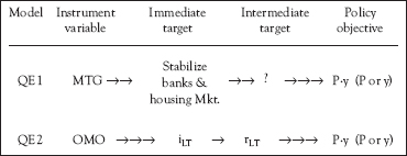
Exhibit 5.2 QE1 and QE2 Transmission Mechanisms
QE2 involved the Federal Reserve purchase of $600 billion of long-term U.S. Treasury securities. The immediate target was to reduce the long-term nominal interest rate (Exhibit 5.2). Although not often noted by the Fed, rational economic agents think in real terms and the intermediate target was a lower long-term real interest rate. The ultimate policy objective was to increase aggregate spending, specifically spending on durable goods which are typically financed with long-term credit.
It is noteworthy that transmission mechanism for QE2 differed from the transmission mechanism for interest-rate targeting, or Model I (pp. 111−112). The immediate target for QE2 was a long-term nominal rate; for Model I, it was the short-term nominal rate. The intermediate target and the policy objective were the same.
The QE2 transmission mechanism had an historical antecedent in the early 1960s. At that time, it was referred to as operation twist. The magnitude of U.S. Treasury security purchases was much more modest in the 1960s, but the motive in both cases was to alter the shape of the yield curve by lowering the long-term interest rate.