CHAPTER 6

Critiques of Monetary Policy

Critiques of Monetary Policy

Fiat money is a relatively new phenomenon. It has been in use slightly more than three-quarters of one century. Thus, how historians will eventually evaluate this experiment with fiat money is yet to be determined. It is probably an understatement to suggest that the U.S. experience with this type of money, to this point, has not been an unmitigated success. Because fiat monies are controlled by governments, what historians must eventually assess is how governments have performed.

Monetary policy is reasonably transparent and the performance of governments as custodians of fiat money has not gone unnoticed. The critiques discussed in the next sections are not concerned with situations where seigniorage is the principal motive of monetary authorities. Rather, the focus is on the practice of discretionary monetary policy in countries where macroeconomic management is the driving force behind policy.

A common thread in critiques of monetary policy is the critical role that knowledge plays in the successful implementation of discretionary monetary policy. The critiques that follow demonstrate the multi-dimensional nature of the knowledge issue.

One very important kind of knowledge required of central bankers is knowledge about the performance of the economy, something that is necessary if monetary authorities are to know whether monetary ease or tighter money is the appropriate policy. When knowledge does exist, it is not always apparent that central bankers will be in a position to utilize that knowledge. Political considerations may interfere. Central banks are also expected to understand how the policy they enact is transmitted to the economy, and how those affected will respond to that policy. Finally, it is important for central banks to know what effect, if any, the infusion of new money has on relative prices and the allocation of resources across markets.

Friedman: Rules vs. Discretion

Milton Friedman argues that the use of discretionary monetary policy has resulted in increased economic instability. The problem is not with the use of fiat money. Rather, it is with the procedures employed by central banks to implement monetary policy, specifically the use of discretionary policy. Replacing that type of policy with a monetary rule would greatly reduce economic uncertainty, especially uncertainty about the future course of monetary policy. This would provide a much better climate for productive activity and eliminate much of the economic instability occasioned by the use of fiat money.

In fashioning this position, Friedman’s posture is diametrically opposed to those who favor the use of discretionary policy. Proponents of discretionary policy maintain that its use can greatly improve macroeconomic performance. Appropriate application of policy instruments will both reduce short-run business cycle fluctuations and bring us greater long-run price stability. Monetary stimulation during a recession, for example, will shorten the recession. If too much inflation is the problem, tighter monetary policy is in order.

Friedman’s case against discretionary policy is that those implementing such policies most often do the wrong thing. Two principal reasons for this are: 1) politics, and 2) ignorance. By doing the wrong thing, those implementing discretionary policies make economic conditions worse rather than better.

Politics

Economic analysis of monetary policy often proceeds as if this policy were conducted in a political vacuum. That decidedly is not the case. Monetary policy is carried out by government, and the political consequences of a policy action receive careful consideration. What is considered rational policy from a political perspective can differ significantly from that implied by economic theory. If political considerations dominate, those implementing discretionary policy may, with good reason, deliberately select the incorrect economic policy.

Political considerations can affect monetary policy even in countries (such as the United States) that have a fairly independent central bank. When, for example, is a good time for the central bank to invoke a tighter monetary policy that results in higher nominal interest rates? From a political perspective, the likely answer is never. As a consequence, central bankers bold enough to undertake such policies can expect politicians to sharply criticize their actions. That may be enough for policymakers contemplating such action to reconsider.

Elections cycles also create problems for those implementing discretionary monetary policy. In the absence of political pressure, introducing a policy change too close to an election can be interpreted as politically motivated. For central bankers in democratic countries who are sensitive to such charges, this might inhibit the implementation of an otherwise appropriate change in monetary policy.

A second way that election cycles influence monetary policy is through the actions of politicians concerned about an imminent election. They might exert pressure on central bankers to undertake policies favorable to their election (or reelection). Research suggests that, in the United States, this may be the rule rather than the exception. For the period from 1951 to the end of the 1970s, Robert Weintraub found that changes in Presidential administrations generally resulted in changes in monetary policy in a direction consistent with the economic views of the President.¹ Given that Ronald Regan ran on a platform of reducing inflation, Paul Volker’s disinflationary policies in the 1980s are an indication that Weintraub’s results extend beyond his sample period.

A prototypical case study in central bank accommodation was President Richard Nixon’s reelection campaign in 1972. Inflation was increasing at the time, and economic theory implied a tighter monetary policy. Tighter money, however, was not the policy of choice for President Nixon. From his perspective, such policies had cost him the Presidential election in 1960. He was not interested in a repeat of that experience. Federal Reserve Chairman Arthur Burns accommodated President Nixon’s desire that monetary policy not be tightened. Nixon won the election, but at a considerable cost to the economy.

Ignorance

A second reason for the failure of discretionary policies is ignorance. The existence of time lags presents a major problem for those attempting to implement discretionary policies. These lags imply that policy carried out today has its impact in the future. Selection of the appropriate policy, then, requires the ability to forecast accurately. Economists, however, are notoriously weak when it comes to forecasting future economic activity. This ignorance is especially pronounced for turning points in the economy, where one would anticipate significant changes in discretionary policy.

Three time lags encountered when implementing discretionary policy are the recognition lag, the execution lag, and the impact lag. To illustrate the difficulties introduced by these time lags, refer to Figure 6.1. Real GDP (y) is plotted against time (t). The business cycle peak occurs at time t₁, with GDP equal to y₁.

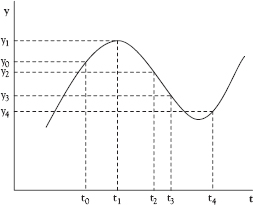
Figure 6.1 Discretionay policy with time lags

The decline in economic activity commencing at time t₁ is not discovered until time t₂. One reason for this lag is that published economic data generally are a record of the past, and turning points in economic activity often are not discovered in these data until well after they happen. For this cycle, the time interval (t₂ − t₁) is the recognition lag. It is the time that elapses between when the economy changes, and when policy makers know about the change.

The policy response is not instantaneous. In the case of monetary policy, the central bank must both adopt a new policy and implement that policy. These events too, require time. Assume that the policy response, which is additional monetary stimulation, occurs at time t₃. The time interval (t₃ − t₂), then, is the execution lag. This is the amount time that elapses between recognition of the problem and when policy makers undertake appropriate policy action.

The impact of this policy action, likewise, is not instantaneous. Rather than occurring at a point in time, it is distributed over a period of time. The precise timing of the impact is unknown. Friedman’s estimates for the U.S. economy are that it will have little (or no) impact for the first 9–12 months, with the total impact occurring over a period of years.

Simplifying, assume that the impact of monetary policy does occur at a single point in time (t₄). By that time, the economy has already entered the expansionary phase of the business cycle. To moderate business cycle fluctuations, this phase of the cycle calls for monetary restraint. Instead of monetary restraint, however, the central bank is providing monetary stimulus. It has done the wrong thing. Monetary policy will accentuate the business cycle upswing and, in doing so, it increases the amplitude of the business cycle.

Given the existence of these time lags, appropriate discretionary policy for this economic cycle requires that the central bank undertake simulative policy before the business cycle downturn occurs, e.g., at time t₀. The wisdom to do so, however, requires that (central bank) economists correctly forecast the impending peak at t₁. Their inability to accurately forecast turning points, or ignorance, generally precludes that.

Friedman’s x-Percent Money Growth. Rule

Even though it is inadvertent, central bank implementation of discretionary monetary policy often makes things worse rather than better. For that reason, Friedman recommends scrapping discretionary policy. In its place, the central bank should follow a rule and increase the money supply at a constant rate. If, for example, a rate of 4% is selected, the central bank increases the money supply 4% each year. That is Friedman’s x-percent money growth rule.

The particular growth rate that is selected is less important than selecting one. A rate in the neighborhood of 4% may be desirable, however, because it approximates the secular growth rate for production. Synchronizing the growth of money and output would permit (proximate) long-run price stability.

Friedman maintains that the potential benefits of employing a monetary growth rule are enormous. The principal one is a more stable economy. A volatile monetary policy contributes to economic instability, thus increasing the amplitude of the business cycle. Use of a monetary rule effectively eliminates this source of cyclical instability.

A second benefit is increased long-run economic growth. As monetary policy becomes more predictable, the uncertainty faced by those in private business is greatly diminished. This lowers the risk premium in interest rates, and will increase the rate of capital formation in the economy. More capital formation leads to increased worker productivity and higher living standards.

Finally, use of a monetary rule will eliminate of secular inflation. Had the Federal Reserve employed such a rule in the past half-century, the great depreciation that occurred in the purchasing power of the U.S. dollar would have been avoided. Elimination of secular inflation will enhance the services provided by money, especially those eroded by unremitting inflation.

Despite these potential benefits, Friedman is aware of the forces militating against adoption of a monetary rule. A major force is the spiritual legacy of the Enlightenment. The great scientific and economic achievements of the past several centuries have nurtured the sense that man has the ability to make things better through manipulation and control. When placed in a monetary context, this perspective makes it easier for central bankers to inspire confidence in their ability to successfully manage monetary affairs.

Public confidence in central bank stewardship is reinforced by central bank resistance to a monetary rule. Given the complexities of a modern economy, central bankers are often given much greater credit for their ability to manipulate aggregate economic activity than is warranted by experience. The general public often basks in the comfort of a central bank that is “in control.” As human beings, it is natural that central bankers find such deference to their skills and influence quite flattering. It is contrary to human nature to expect them to embrace the prospect of replacing their reasoned judgments with a mechanical procedure that greatly diminishes their social significance.

The Road Not Taken: A Friedman Case Study

It is not possible to know what would have happened had the Federal Reserve followed Friedman’s x-percent money growth rule. That is a road not taken. It is possible, however, to simulate what Friedman had in mind through the prism of the dynamic version of the equation of exchange. In Table 6.1, that relationship is utilized to compare actual data for the 53-year period from 1959–2012 with hypothesized data using Friedman’s x-percent growth rule.

Table 6.1 Dynamic Equation of Exchange for the U.S. Economy (Average Annual Growth Rate: 1959–2012)

Source: Actual U.S. Data: Federal Reserve Bank of St. Louis data base (FRED)

From 1959–2012, annual U.S. money growth (dM₂/M₂) averaged 6.9%. Long-run velocity was relatively stable, declining at an average annual rate of 0.2%. Real Gross Domestic Product growth (dy/y) averaged 3.1%. With too much money chasing too few goods, the United States experienced an average secular inflation rate (dP/P) of 3.6% per year.

By comparison, assume the Federal Reserve implements Friedman’s x-percent growth rule by increasing the money supply by 4% each year. The velocity of money is relatively stable with the assumed annual growth rate (dV/V) the same as the actual growth rate for 1959–2012: −0.2%. Friedman argued that such monetary stability would lead to higher economic growth. Accordingly, the average annual growth rate for real GDP is 4.1%. That was the actual rate of growth for the 1950s, the decade prior to the implementation of Keynesian economic policies during the J.F. Kennedy administration.

For the period under consideration, Friedman’s x-percent money growth rule yielded long-run price stability. Prices, on average, declined 0.3% per year. Such price stability is comparable to that experienced by the United States when the country was using fiduciary money (prior to 1933).

Had the United States actually experienced such price stability, the considerable erosion in the services provided by money would probably not have occurred. For example, with long-run price stability, money would have continued to serve as a viable store of value. In addition, Friedman would likely make the case that United States would have been spared the dislocations and economic hardships associated with the Great Inflation of the 1970s and the ensuing disinflation of the 1980s. He also might argue that, with the x-percent money growth rule, the United States would not have suffered through the Great Recession of 2008–2009. A policy of providing new money at a steady rate (instead of pushing short-term interest rates close to zero for an extended period) would reduce the likelihood of an asset bubble in housing that was at the epicenter of the Great Recession.

Interest Rate Targeting

Central banks in relatively advanced countries generally employ interest rate targeting to implement discretionary monetary policy. Excluding the four-year interlude from 1979–1983, the Federal Reserve System in the United States has targeted interest rates for several decades. While the analysis that follows applies to interest rate targeting more generally, the issue is framed within the context of U.S. monetary policy.

Federal Reserve interest rate targeting conforms to the transmission mechanism described as Model I in the previous chapter. The instrument variable is open market operations (OMO). The immediate target is the short-term interest rate (i_st). The rate selected for this purpose is the federal funds rate, or the rate on immediately available funds. While it is a nominal interest rate, the intermediate target is the long-term real interest rate (r_lt). The ultimate policy objectives are the price level and aggregate spending.

The Fed encounters two very difficult problems when attempting to implement policy through this transmission mechanism. First, it is using a nominal interest rate target in a world where rational economic agents think in real terms. The interest rate of importance, then, is the unobservable real interest rate. Second, the transmission of monetary policy occurs across the term structure of interest rates. The immediate target is a short-term interest rate, but the critical variable is the long-term rate of interest.

The Nominal/Real Dichotomy

The success of Federal Reserve monetary policy is contingent upon control of the real interest rate. Rational economic agents on both sides of the credit market think in real terms and, if one is to change their behavior through policy, it is the real interest rate that counts. Unlike the nominal interest rate, however, the real interest rate is unobservable. The difficulty presented here is that one cannot readily control something that does not lend itself to measurement. That problem is compounded when precision is required. That is generally the case, however, because policymakers employing nominal immediate targets most often change those interest rate targets in increments of one-quarter to one-half percent.

Control of the unobservable real rate of interest is hypothesized to occur via changes in the Federal Reserve’s nominal interest rate target (the federal funds rate). As noted in Chapter 3, however, the nominal rate of interest, too, is comprised of nonobservable components: inflationary expectations; default, money, and income risk premiums; and, time preferences. Each of these components reflects the subjective valuations of millions of market participants. Because subjective valuations of individual economic agents are prone to change, one must operate on the premise that they do. That is, inflationary expectations, risk premiums, and time preferences are incessantly changing.

If these nonobservable components of the nominal rate of interest are unstable, when the Fed changes its nominal interest rate target, it cannot know whether the real interest rate is increasing, falling, or staying the same. If a policy-induced higher real interest rate indicates a tighter monetary policy, and a policy-induced lower real rate the opposite, the Federal Reserve does not know whether its monetary policy is tighter, easier, or neutral.

To illustrate, three different scenarios are presented in Table 6.2. They are designated as Cases I, II, and III. The first scenario (Case I) is the initial condition. The nominal interest rate is 5%, which is also the Fed’s targeted interest rate. With a 2% expected rate of inflation, the real interest rate is 3%. The latter is apportioned into a risk premium and a marginal rate of time preference.²

Table 6.2 The Nominal Interest Rate and Its Components

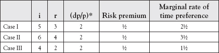
Assume, initially, that the Federal Reserve attempts to tighten monetary policy. In Case II, it raises its target for the nominal interest rate to 6%, and provides reserves less liberally to the banking system. With tighter credit conditions, the nominal rate increases to the desired level. Assuming no change in inflationary expectations, the real rate increases to 4%. The higher real rate of interest leads to reduced capital goods expenditures, and a higher marginal rate of time preference. In this scenario, the Fed thinks that monetary policy is tighter and, indeed, it is. This is how monetary policy with interest rate targeting is supposed to work.

With the subjective preferences of economic agents constantly changing, however, the world is much more complex than this. For example, do these Case II numbers still constitute tighter monetary policy if the higher real interest rate would have occurred as a result of market activity alone? Commence again with Case I initial conditions, i.e., i = 5% and r = 3%. Now, assume an increasingly robust economy with businessmen becoming more optimistic. Their increased time preferences for current expenditures are expressed in the form of a greater demand for capital goods. Tighter credit conditions lead to a higher nominal rate (6%) and a higher real rate (4%). Case II numbers again prevail.

Superimpose upon these events an increase in the Federal Reserve’s target for the nominal interest rate—from 5% to 6%. The Fed’s objective is to increase the real interest rate by 1% (from 3% to 4%). In this case, the Fed does not need to adjust how it is providing reserves to the banking system. The higher interest rates come about through market activity alone, and do not reflect any change in Fed policy. When the Federal Reserve adjusts its interest-rate target upward, that target is simply following the market rate.

This is a case where the Federal Reserve thinks monetary policy is tighter when, in fact, it is not. Errors of this kind are likely when the real interest rate follows a pro-cyclical pattern. If business managers and consumers become more optimistic during a business cycle expansion, their greater optimism is expressed in the form of an increase in their time preferences for current expenditures. The real (and nominal) interest rate rises. If the Federal Reserve simultaneously becomes concerned about the exuberant economy, it will move to tighten monetary policy. As in the example above, however, it will erroneously interpret the market-driven rise in interest rates as policy-induced.

The Federal Reserve is prone to making the opposite kind of error when the economy is contracting. Business managers and consumers become more pessimistic. They experience decreases in their time preferences for current expenditures, and the real (and nominal) interest rate falls. The Fed, in an attempt to stimulate aggregate demand, lowers its interest rate target. With the nominal and real rate already falling, the Fed is unable to distinguish market-induced declines in rates from those occasioned by Fed policy.

This scenario is captured in Case III (Table 6.2). Commencing with the initial condition (Case I), declines in the real and nominal rate occur in response to reduced time preferences. The nominal rate falls from 5% to 4%; the real rate, from 3% to 2%. Simultaneously, the Federal Reserve lowers its target for the nominal interest rate from 5% to 4%. Its intent is to lower the real rate by a similar amount (from 3% to 2%). The Federal Reserve does not need to adjust its provision of reserves to the banking system, because both the nominal and real rates reach their targeted levels through market activity. This is a case where the Fed thinks that monetary policy is easier when, in fact, it is not.

Thus, there are serious reservations concerning the Federal Reserve’s ability to effectively control the real rate of interest. When the Fed changes its nominal interest rate target, it does not know with any assurance either the magnitude or direction of policy-induced changes in the real rate of interest.

The Term Structure Problem

A second problem the Federal Reserve confronts when targeting interest rates relates to the term structure of interest rates. Not only does the Fed not know whether adjustments in its immediate target result in the desired change in the real interest rate, but those policy changes also must be transmitted across the term structure of interest rates. The Federal Reserve’s operating target is the short-term nominal rate, but its intermediate target is the long-term real interest rate.³

The rationale for this transmission mechanism (Model I) is discussed in Chapter 5. Outlays for durable goods, both business and consumer, are more easily deferred than are expenditures for nondurable goods. As a consequence, durable goods account for much of the volatility in aggregate spending. Attempts by policy makers to influence aggregate spending (and the price level), then, are geared towards controlling expenditures for those types of goods. With durable goods purchases frequently financed through the issue of long-term bonds, those purchasing durable goods are sensitive to the long-term rate of interest. It follows that, when the Fed employs interest rate targeting, it must target the long-rate.

Precisely how the Federal Reserve successfully navigates the term structure and, simultaneously engineers changes in the real interest rate, is not clear. Moreover, various theories of the term structure (discussed in Chapter 3) do not provide much help. If anything, they cast additional aspersion upon the Fed’s ability to successfully implement discretionary policy through interest-rate targeting.

Explanations based on the segmented markets hypothesis, for example, are not encouraging. If market participants adhere strongly to their maturity preferences, there is little likelihood that policy-induced changes in the short-term interest rate target will be transmitted across the term structure to long-term rates of interest. Federal Reserve control, in turn, is marginalized.

On the other hand, information requirements implied under the unbiased expectations and the liquidity preference theories present an even more serious obstacle for those conducting monetary policy. First, the Fed must have prior knowledge of the term structure of inflation premiums and the term structure of risk premiums. Second, it must know how those term structures are changing independent of monetary policy. Finally, it must also know how a given change in its short-term interest rate target will affect both of those underlying term structures. Compounding the Fed’s information problem is the fact that both inflationary expectations and risk premiums are imbedded in the term structure of interest rates, and not directly observable.

It is clear that the U.S. central bank faces serious information problems when attempting to target long-term real interest rates through use of a short-term nominal operating target. If the Federal Reserve acts as if it can orchestrate desired changes in aggregate spending and the price level through this procedure, it is committing what Friedrich von Hayek called “the pretense of knowledge.”⁴ It is pretending to know things that, in fact, it does not.

A Recent U.S. Case Study

This knowledge problem confronting the Federal Reserve is a good illustration of what happens when the criteria for selecting monetary targets (discussed in the previous chapter) are not satisfied. Because it is not possible to accurately measure the long-term real interest rate, the Federal Reserve is employing a target it cannot control. Moreover, lack of knowledge of the long-term real rate also means the linkages in Model I are not predictable.

U.S. monetary policy from 2004–2006 exemplifies the difficulties encountered when these monetary target criteria are not met. Starting in June, 2004, the Federal Reserve increased its target for the federal funds rate fifteen consecutive times. As a consequence, the federal funds rate target in April, 2006 was 4.75% versus 1.00% in the first half of 2004. Those changes are chronicled in Table 6.3.

Table 6.3 Federal Funds Rate Target

Date	Level (percent)
2006
March 28	4.75
January 31	4.50
2005
December 13	4.25
November 01	4.00
September 20	3.75
August 09	3.50
June 30	3.25
May 03	3.00
March 22	2.75
February 02	2.50
2004
December 14	2.25
November 10	2.00
September 21	1.75
August 10	1.50
June 30	1.25
2003
June 25	1.00

Source: Board of Governors of the Federal Reserve System

Many observers routinely describe these upward adjustments in the federal funds rate target as tighter monetary policy. There are serious doubts, however, about such an interpretation. It is true that other short-term nominal rates increased along with the federal funds rate. The three-month Treasury-bill rate, for example, rose from 1.17% to 4.60% between June 1, 2004 and March 1, 2006.⁵

But, as previously noted, higher short-term nominal interest rates do not necessarily mean tighter monetary policy. Long-term nominal interest rates actually fell during the same 21-month period. The rate for 20-year U.S. Treasury securities declined from 5.45% to 4.74%. These changes in both long-term and short-term rates for U.S. Treasury securities are reflected in Figure 6.2. It depicts the shapes of the term structure of interest rates for U.S. Treasury securities on both June 1, 2004 and March 1, 2006. The yield curve in 2006 became noticeably flatter.

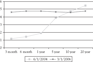
Figure 6.2  Term structure of interest rates US treasury securities: Constant maturity

Source: Board of Governors of the Federal Reserve

Lower long-term nominal interest rates, however, are not the issue. It is long-term real interest rates, and not nominal rates, that are critical for economic decisionmakers. If monetary policy was, indeed, tighter during this 21-month period, long-term real interest rates must have increased while nominal rates were falling. Moreover, the increase in real rates must have occurred as a result of monetary policy and not due to other factors such as an increase in default risk or changes in time preferences for current expenditure. While such a scenario appears doubtful, no one knows for certain. Hence, the appropriate answer to the question about whether monetary policy is tighter is: “I don’t know.”

Monetary Aggregates and Monetary Control

Recent Issues with Monetary Control

After facing difficulties with interest-rate targeting during and after the Great Recession (2008–2009), the Federal Reserve embarked on several massive asset purchase programs described as quantitative easing. Those carried out during the Great Recession are discussed in Chapter 5 (pp. 118–119).

While the Fed’s asset purchase programs were not advanced with the stated intent of increasing monetary aggregates, they did. In doing so, these programs raised an additional issue relating to central bank control of the money supply. These issues are discussed in the context of the general money supply model in Chapter 4 (equation 4.2).

The magnitude of the Federal Reserve’s asset purchases caused the monetary base in the United States to explode. Base money increased more than threefold from 2007 and 2012, and was largely in the form of increases in bank reserves. Under more normal circumstances, one would anticipate a massive increase in the money supply, huge increases in spending, and the potential for the largest inflation in U.S. history.

To date, none of these things have happened. The reason is that banks have not used this infusion of bank reserves to extend additional bank credit (and expand deposit money). Instead, those reserves were almost entirely held in the form of excess reserves.

In the money supply model, an increase in the aggregate bank excess reserve ratio causes the money multiplier to decrease. In this case, because the increase in bank excess reserves was so massive, the multiplier collapsed.

As shown in equation 6.1, the large increase in the monetary base was virtually entirely offset by a fall in the money multiplier. In the context of these changes the consequences for money (which did rise) were minimal.

This experience has important implications for monetary policy. It differs from the liquidity trap explanation advanced by early Keynesians. In that case, the central bank increases the money supply and it has no effect on spending. People hold rather than spend the additional money, and velocity falls. When this happens, monetary policy is ineffective.

In the present case, the effectiveness of monetary policy is questioned for a different reason. Unlike the previous case, the money supply does not increase, or it does so minimally. What distinguishes the recent experience is collapse of the money multiplier as shown in 6.1.

The precipitous fall in the multiplier represents a breakdown in a transmission mechanism for monetary policy. In Chapter 5, the transmission mechanism employing monetary aggregates as targets was Model II. In that transmission mechanism, what links base money to the money supply is the base money multiplier. The usefulness of that transmission mechanism is predicated upon a predictable relationship for transforming base money into money. It is that relationship that fell apart.

This experience raises serious questions concerning the ability of the Federal Reserve to control the money supply. When combined with the lackluster results from interest rate targeting, it appears that both transmission mechanisms I and II for implementing discretionary monetary policy did not perform as expected during and after the Great Recession (2008–2009).

Why the Federal Reserve Needs an Exit Strategy

The massive infusion of bank reserves (and base money) into the U.S. financial system from 2008 to the present leaves the Federal Reserve with an important legacy issue. If the United States is to avoid significant future inflation, the Fed must undertake future monetary policy that (largely) removes that base money from the system or, alternatively, provides banks with an incentive to not activate the massive excess reserves they now hold. The description of how the Federal Reserve plans to do this is known as the Fed’s exit strategy.

The magnitude of the problem confronting the Federal Reserve is apparent in Table 6.4. From 2007–2012, bank reserves and base money increased by 1,611% and 213%, respectively. These dramatic increases were not reflected in the money supply (M₂) which rose by only 37.7%. This surprisingly modest number is the result of the collapse of the base money multiplier (m), which fell by 57.5%. These data comport with the directional changes in equation 6.1 above.

Table 6.4 Bank Reserves, Base Money, Money Supply, and the Money Multiplier for the United States 1999–2012

Source: Monetary Trends, (various issues, Federal Reserve Bank of St. Louis)

The problem confronting the Federal Reserve is about what happens in the next business cycle expansion. Since the most recent business cycle trough (June, 2009), businesses and households have behaved very cautiously. Credit demands by both sectors have been restrained, and economic growth has been tepid.

If, in the future, both businesses and households throw caution to the wind, and become very aggressive in their demands for credit, banks (which are awash in liquidity) are in a position to accommodate them. Moreover, banking competition makes them inclined to do so. If an individual bank refuses a customer’s demand for credit, that customer is likely to take his/her banking business to another bank.

Meeting these credit demands means an increase in money growth, which has the potential to accelerate sharply. The acceleration in money growth, in this case, is occasioned by an increase in the base money multiplier. As banks reduce their holdings of excess reserves, the aggregate excess-reserve ratio falls and the money multiplier rises.

The potential impact on the money supply is captured by assuming that the multiplier returns to its prerecession level of 8.54 (2007). If that adjustment had occurred in 2012, the impact on the money supply for that year is shown in 6.2.

With a multiplier of 8.54 in 2012 (and assuming the same 2012 level for base money), the money supply would have been $22,733.5 billion for that year instead of the recorded level of $10,006.4 billion. That represents a 127.2% increase in the money supply. In other words, the money supply has the potential to grow this much if the multiplier were to return to its prerecession level. If all of this money growth were to occur in a single year, the average price would increase by a magnitude of the same order.⁶ Thus, the potential exists for much higher inflation than occurred in earlier episodes such as the Great Inflation of the 1970s. That is why the Federal Reserve needs an exit strategy.

Rational Expectations

Economists know that a person’s expectations affect the economic decisions made by that individual. Rational expectations theory is concerned with how those expectations are formed and, also, how economists model those expectations. Much of this theory was developed in response to the use of large macroeconometric models (by business and government). Statistical in form, these models were an adjunct to the Keynesian revolution in macroeconomic theory. The models often contained several hundred equations, and were used for forecasting purposes. Keynesian economists used the models to advise governments about the consequences of different activist policies, while those in the private sector used them as an aid in business decision-making.

Many of the equations in macroeconometric models were behavioral in nature. That necessitated the modeling of expectations, even though those expectations were unobservable. Proxies for these unknown expectations were most often obtained by assuming that economic agents have adaptive expectations. With this approach, the expected value of a variable was estimated as a weighted sum of past values of that same variable. Historical time series data were employed for rendering concrete estimates.

Econometric models constructed using this methodology often result in large forecasting errors, and economists in the rational expectations tradition have a ready explanation for this. Reliance on adaptive expectations as a proxy for actual expectations is an inherent weakness of the models. For, modeling human behavior in this way is tantamount to assuming that economic agents are irrational. The reason is that economic agents with adaptive expectations make systematic errors. That is, they repeatedly make the same mistakes.

An alternative to assuming that expectations are adaptive is to assume they are rational. Rational individuals are not restricted to using past information (such as past values of variables) when forming their expectations. Their expectations are formed by taking into account all information that is worthwhile acquiring. Agents behaving in this fashion are said to have rational expectations. Once the models of economists incorporate rational expectations, economic agents are less prone to making the same mistakes repeatedly—systematic errors. Moreover, such rational behavior has implications for the effectiveness of economic policy.

If economic policy affects economic agents in a significant way, then it is rational for them to take the effects of that policy into account. Furthermore, if those administering policy behave consistently, economic agents will learn how that policy is implemented under different economic circumstances. Once they do, individuals will adjust their behavior to the policy, and make necessary behavioral changes before any change in policy is undertaken. Because adjustment to the policy has already taken place, no behavioral response follows any predictable change in economic policy. In rational expectations theory, this result is known as the Policy Impotence Theorem.

When behavior is rational in this sense, discretionary policy loses its effectiveness. An example of such policy impotence in the context of rational economic behavior is chronicled in Table 6.5. In Period I, individuals anticipate monetary ease that will occur in Period II. Sensing that they will be able to finance additional expenditures at a lower rate in the near future, they adjust their current expenditures upward. Producers respond by increasing production in Period I and, in the absence of a change in the money supply, the offsetting entry in the equation of exchange is an increase in the velocity of circulation of money (V↑).

Table 6.5 Policy Impotence Theorem

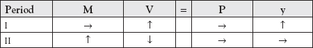
In period II, the central bank increases the money supply to stimulate aggregate demand. However, there is no increase in spending because rational economic agents anticipated this monetary stimulation and have already adjusted their spending plans (in Period I). In Table 6.5, the money supply increases in Period II but GDP expenditures remain the same. The offsetting entry is a decline in velocity (V↓). The monetary ease engineered by the central bank in Period II has no effect on current spending, i.e., it was impotent.

The rational expectations argument against the use of discretionary policy does differ from that of Friedman (and the monetarists) in one important respect. In Friedman’s case, discretionary policy does not work because policymakers are either ignorant or subject to political influence. For the rational expectations economists, discretionary policy does not work because those affected by the policy are the opposite of ignorant. They are too smart (or rational).

The Austrian Perspective on Monetary Policy

Economists in the Austrian tradition generally favor “hard money.” They find it vexing that a monetary economist such as Milton Friedman favors reliance upon markets everywhere except in his area of expertise, the realm of money. The Austrian position is that money is too important to be left to government. Instead, money and all monetary relations should be determined through exchange activities in the marketplace. Because fiduciary money was a spontaneous market development, and fiat money was not, Austrians generally favor reestablishing fiduciary money by returning to the gold standard.

If the quantity of money and all monetary relations are determined by market participants, government has no monetary role. There is no monetary policy. For that reason, Austrians are against all monetary policy as practiced under fiat money regimes. That would include Friedman’s monetary growth rule as well as all variations of discretionary policy.

At the center of the Austrian critique of monetary policy is the concept of the price level. The importance attached to the idea of an average price dates back to the early 20th century, when Irving Fisher argued that the value of money should be standardized.⁷ By this, he meant that the objective of government monetary policy should be to stabilize the average price, or the price level. While Fisher was unsuccessful in his crusade to standardize money, the concept of the price level subsequently assumed a life of its own. After governments mandated the use of fiat money, the price level became a variable subject to manipulation by monetary authorities.

Despite the efforts by central banks to manage the price level, Austrians give the concept little credence. For them, the price level has no significance independent of its component parts—the individual prices. To the extent that there is an average price, it is an aggregation of these individual prices. In a market setting, each individual price has meaning, or informational content. Each is an expression of the subjective valuation that individuals have placed on that object. Viewed collectively, a set of individual prices represents relative valuations.

With no rigid dichotomy separating microeconomics and macroeconomics, the significance Austrians attach to individual prices is not restricted to the realm of microeconomics. They are equally important in a macroeconomic setting. Hence, when central banks manipulate the price level, without regard to its constituent parts, they destroy the informational content of individual prices. In doing so, they disrupt the critical role that prices play in coordinating the diverse economic activities that collectively make up the aggregate economy.

Assume, for example, that a central bank employs monetary policy to stabilize the average price. The problem here is that market participants may have preferences that are not consistent with an unchanged exchange value for money. In the absence of monetary policy, they may have valued money either more highly or less highly than before. If they valued money more highly, their preferences were consistent with deflation rather than price stability. Alternatively, placing a lower value on money would result in inflation.

When money is a strictly a market phenomenon, inflation, deflation, and price stability are all possible outcomes. Moreover, there is no analytical basis for favoring one of these outcomes over the others. This view is antithetical to conventional thinking, especially with regard to deflation. Most contemporary policymakers, and many economists, consider deflation highly undesirable—something that must be avoided at all costs.

The source of this bias against deflation is the Great Depression experience, when deflation was accompanied by an unprecedented drop in production. To generalize from this episode, however, is ahistorical. Data generally do not affirm such a linkage between deflation and economic decline.⁸ Moreover, given our experiences with fiat money, it seems much more likely that massive economic decline would be accompanied by significant inflation rather than deflation.

In contrast to the conventional view, Austrians do not readily dismiss deflation when it is the natural outcome of economic activity. Deflation generally occurs when a country’s growth rate for production exceeds the growth rate of money. Money becomes more scarce in relation to goods, and that tends to occasion an increase money’s exchange value. This happened in the United States during the last third of the 19th century. The country was on the gold standard, and there were few new discoveries of gold to augment the world’s gold supply.

Data for this period, assembled by Christina D. Romer, appear in Table 6.6. Deflation averaged 1.36% per year from 1869 to 1899. In contrast to the conventional view of deflation, this period of falling prices was not one of economic calamity, or even malaise. Instead, it was a period characterized by much innovation and very rapid industrialization. The average growth rate for production was considerably higher than average growth during the 20th century. Moreover, production growth was, by far, most rapid in the decade with the highest rate of deflation (1869–1879).

Table 6.6 Prices and Production in the United States: 1869–1899 (percent change)

Year	Real GNP	GNP-Implicit price deflator
1869-1879	5.38	-3.23
1879-1889	3.21	0.03
1889-1899	3.82	-0.85
1869-1899	4.13	-1.36

Source: Romer (1989), pp. 1–37.

Historical episodes like this suggest that changes in the general price level (such as inflation or deflation) generally do not cause problems when they are driven by market forces. A collateral issue, though, is whether problems arise when the source of the price-level change is monetary manipulation by the central bank, and not market adjustments occurring in response to changing market conditions.

Austrians answer this question in the affirmative. Consider, initially, what happens when changes in the quantity of money are a derivative of the market process. Allocation of additional resources to the production of new money, in this case, originates with decisions made by individual market participants. As a response to market demand, the additional money was, in a sense, “ordered” by those market participants. It reflects their preferences concerning the use of scarce resources. Any change in prices brought about by the new money is, likewise, a part of the same market process whereby individual plans and preferences are rendered consistent with one another.

The situation is entirely different when the source of a change in money is the central bank. In this case, the additional money is not ordered by market participants. As a consequence, it is not a part of the market adjustment process that renders individual plans consistent with one another. Instead, the new money is a disruptive force in markets. By changing relative prices, compared to what they otherwise would have been, it destroys the informational content of market prices. Relative prices no longer represent that delicate balance necessary to coordinate economic activity across markets.

A critical price often distorted by monetary policy is the real interest rate. This rate reflects the time preferences of market participants. A given real rate specifies how much future consumption economic agents are willing to sacrifice in order to have more present consumption. By affecting how consumers distribute consumption across time, the real interest rate plays an essential role in the intertemporal allocation of resources.

When monetary policy brings about a change in the real interest rate, it adversely affects the intertemporal allocation of resources. It does so by distorting the informational content present in a market-determined real rate of interest rate. The new real interest rate occasioned by monetary policy emits the “wrong” signal to market participants, and the economic coordination brought about by market prices is disrupted. Production plans of firms are no longer consistent with the preferences of their customers.

The disruptive influence of monetary policy is illustrated by comparing situations with and without monetary policy. The market under scrutiny is the loanable funds market. Prior to the introduction of monetary policy, the real interest rate plays its allocative role. In doing so, it renders the plans of all economic agents consistent with one another. Those plans are reflected in the demand and supply curves D and S in Figure 6.3.

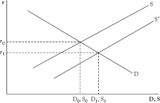
Figure 6.3  Market for loanable funds

Plan consistency occurs at the market clearing rate r₀. The quantity of loanable funds supplied, S₀, shows abstinence from present consumption by economic agents. It is exactly equal to the quantity of loanable funds demanded, D₀. This demand originates with consumers desirous of consuming more than their incomes, and producers borrowing to acquire capital goods.

Intertemporal economic coordination occurs in this case because the real interest rate is transmitting the correct information to market participants. The amount of resources released from (net) present consumption is precisely absorbed by those borrowing to purchase capital goods. Those abstaining from present consumption are choosing an increased amount of future consumption. That demand for future consumer goods will be accommodated by a larger volume of future output made possible by current capital formation.

Such intertemporal coordination of economic activity no longer prevails once monetary policy is introduced. The reason is that the information contained in the real interest rate is distorted by monetary policy. To show this, assume the central bank increases the money supply. The supply curve for loanable funds shifts to the right (to S ′). There is now an excess supply of loanable funds at r₀, and the real interest rate falls to r₁.

While this lower real interest rate does clear the credit market, the rate did not fall due to any change in the plans of individual economic agents. It did not fall, for example, because consumers desire to defer more consumption to the future, or because producers choose to purchase fewer capital goods. A lower real interest in either of those circumstances would convey such a change in preferences to others in the market.

Instead, the source of the decline in the real interest rate is the additional funds made available through monetary policy. By falling without any changes in the plans of economic agents, the informational content of the real interest rate is compromised. At r₁, the real interest rate is below the level (r₀) that renders the diverse plans of economic agents consistent with one another. The new real interest rate is transmitting the wrong signals to market participants.

Producers are encouraged to purchase more capital goods, and they bid the necessary resources away from those producing consumer goods. The problem is that this redirection of resources is not consistent with consumer preferences. Consumers have not chosen to tradeoff additional present consumption for more future consumption. This miscommunication brought about by monetary policy has important macroeconomic consequences. At some point, this misallocation of resources will have to be rectified. The endplay involves economic recession with all of its attributes—falling (and possibly negative) profits, idle capital goods, unemployment, and business bankruptcies.

From the Austrian perspective, then, all monetary policy is disruptive rather than beneficial. It destroys the informational content of market prices. Unfortunately, to undo the pernicious effects of such policy is not a costless proposition. Requisite adjustments in the allocation of resources are similar to those that are necessary at the end of a protracted war. Large quantities of resources are misallocated in the sense that they are used to produce war materials that are no longer useful. These situations often lead to a period of falling output and increased unemployment.

Case Study: Federal Reserve Policy and Malinvestment

Austrian economists make the case that recent Federal Reserve policy is instructive for understanding the nature of boom/bust cycles. First and foremost, such cycles are generated by central banking policy. In that context, the Great Recession of 2008–2009 is viewed as a prototypical business depression emanating from prior interest rate policies of a central bank, in this case the Federal Reserve.

In the first decade of this century, Federal Reserve policymakers were convinced that the U.S. economy was facing the specter of deflation. As noted earlier, such a prospect is generally viewed by those implementing monetary policy as an anathema. The Federal Reserve reacted accordingly.

The antidote for deflation was an increase in aggregate spending. From the Federal Reserve’s perspective, lower interest rates were in order. That they engineered. The target rate for the federal funds rate was reduced sharply, and eventually held at 2.0% or less for more than three years—from November, 2001 to December, 2004. The intent was to defuse deflationary forces by encouraging greater spending on durable goods.

The problem, from an Austrian perspective, is that interest rates are something more than prices subject to manipulation by the Fed. They are critical for the intertemporal coordination of economic activity. By manipulating interest rates, the Federal Reserve destroyed the informational content of market prices and disrupted the allocation of resources across time.

The policy-induced lower interest rates encouraged more roundabout productive activities, i.e., a greater production of durable goods. That, indeed, was the Fed’s intent. The difficulty is that consumers did not, through their market activity, initiate the order for these additional capital goods. They came about because consumers were reacting to a false set of prices engineered by the central bank.

In this episode, a sizable portion of the addition to the country’s capital stock was in the form of new housing. The housing boom contributed, temporarily, to a more robust level of economic activity. That boost in activity was not to be permanent. From the Austrian perspective, the bloated housing stock was a manifestation of a previous misallocation of resources—one induced by Federal Reserve policy. It is what Austrians refer to as malinvestment. The market correction, or the bust, played out as the Great Recession of 2008–2009.

Postscript

These critiques provide insight into the kinds of problems confronting modern governments as they manage fiat money systems. Collectively, they explain why those charged with that responsibility often perform poorly and sometimes fail. Their task is a daunting one. As an indication, critics cite the following skills and/or conditions as those most likely to result in a favorable discretionary monetary policy experience.