CHAPTER 4

Central Banks and the Money Supply

Banks, Bank Lending, and Money

Commercial banks are profit-oriented depository institutions. Bank customers place deposits with these institutions, and also use these bank deposits to make payments. That is, banks deposits are used as money. Since the bulk of the money supply resides in commercial banks, banks are often viewed as custodians of our money supply.

Commercial banks have an even larger monetary role because they are a conduit for the implementation of monetary policy. Currently, the most common way for the money supply to increase is through bank lending. When a bank makes a loan, the proceeds of the loan are in the form of an increase in the customer’s deposit balance at the bank. Payment in this form is satisfactory to the bank customer because bank deposits are used as money. The customer can now spend this new deposit to purchase the item he/she is financing through credit.

The impact of the bank loan on the balance sheet of the bank is shown as transaction 1) in Exhibit 4.1. Bank A, the lending bank, has an additional loan in its portfolio (Loan +). The offsetting liability entry is the increased deposit balance of the borrowing customer (DD√ +).

Exhibit 4.1 Bank Loan

When Bank A extends credit to a customer in this fashion, the money supply increases. That is because the proceeds of the loan is new deposit money. The aggregate money supply is now higher than it was before. Bank A now holds more deposit money. Every other bank in the system has the same amount of deposit money as before. Changes in the money supply are shown in equation 4.1.

The reason that banks make loans to their customers is that it is profitable to do so. Assume that the interest rate on the loan made by Bank A is 5%. Assume, as well, that DD√ is a noninterest bearing deposit account. The spread on this loan is 5%. If the customer does not default on the loan, this is a profitable transaction for the bank.¹

Given the profitability of such loans, the question is why the Bank A does not make a zillion loans. The answer is that Bank A’s lending is constrained by the availability of its bank reserves. That is apparent once the customer borrowing from Bank A spends that newly-created money, e.g., the customer purchases a house. If the person selling the house banks at another bank, Bank B, money for the home purchase is now transferred (through the payments system) from Bank A to Bank B. Thus, while the newly-created money by Bank A is not lost to the banking system, it is lost to Bank A. Bank reserves follow the deposit money to Bank B when the check for the home purchase clears. That is, when Bank A repatriates (through the clearing system) the check for the home purchase, it gives reserves in exchange for the check. Transaction 2), in Exhibit 4.1 shows the loss of reserves at Bank B as well a reduced deposit liability. The latter occurs when the check for the house purchase is cancelled.

The results of combining transactions 1) and 2) appear in Exhibit 4.2. Bank A has an additional asset in the form of a bank loan. It acquired the asset through the loss of bank reserves. Thus, when a bank makes a loan, it can expect to lose reserves in the amount of the loan. It is the availability of bank reserves, then, that constrains the volume of lending undertaken by an individual bank.

Exhibit 4.2 Net Effects of a Bank Loan

Acquiring bank reserves is important to banks. An individual bank can increase its reserves in a number of ways. In competition with other banks, it can lure more customers. When they deposit, they bring reserves. A bank can also liquidate other assets that it holds in order to augment its reserves. Another potential source of bank reserves is through issuing liabilities, e.g., by borrowing reserves in the federal funds market.

Each of these cases is a zero-sum game. When one bank gains reserves, another bank in the system loses reserves. Net additions to bank reserves for all banks collectively most often originate through monetary policy. The model of the money supply presented in the next section allows for the investigation of both sources and uses of bank reserves. The techniques employed by central banks to increase the total quantity of bank reserves are integrated into the model.

A Model of the Money Supply

This money supply model is used to examine factors that determine the total quantity of money. In its basic form, the components are the level of base money (B), the base money multiplier (m), and the quantity of money (M). The model is presented in the form of both levels and differences (absolute changes).

Equation 4.2 states that the level of money (money supply) is equal to the level of base money (monetary base or high-powered money) times the level of the base money multiplier. Equation 4.3 expresses the same relationship in terms of differences. The change in the money supply (dM) depends on changes in the monetary base (dB) and changes in the money multiplier (dm). The M1 measure of money is used in this chapter, although it is possible to use the same general model for other measures.

Base Money

The monetary base is the primary form of money. It varies with the type of money used, and generally serves as the foundation for other elements of the money supply. In the case of commodity money, the levels of M and B are the same. Assume, for example, that gold coins are the only form of money. These gold coins serve as the monetary base. Base money is equal to the total quantity of gold coins (G), which is also the level of the money supply. With B and M the same number (equation 4.4), the money multiplier assumes the trivial value of one. Exhibit 4.3 shows the value of the money multiplier under different monetary systems.

Exhibit 4.3 Values for m Under Different Monetary Systems

With fiduciary and fiat monies, the size of the money multiplier depends upon whether banks practice 100% reserve banking or fractional reserve banking. 100% reserve banking is when a banking institution holds bank reserves in the proportion of 100% of its deposit liabilities (Bank reserves are the cash holdings of a bank). With fractional reserve banking, a bank’s cash reserves are less than 100% of its deposit liabilities.

Fiduciary money is a hybrid arrangement. It consists of an underlying commodity money, and fiduciary elements that are convertible into commodity money on demand. Assuming again that the commodity money is in the form of gold coins, the total quantity of these gold coins (G) is the monetary base. There are now alternative uses of the monetary base. A portion is used as circulating money (G_M); the remainder, as bank reserves (G_B). This partition appears in equation 4.5.

The total money supply (equation 4.6) is equal to the quantity of circulating gold coins (G_M) plus the quantity of circulating fiduciary money (FG_M) that is convertible into G_M. Fiduciary money is issued by banking institutions. With 100% reserve banking, G_B = FG_M. Consequently, M = B, and the size of the money multiplier is one. Banks are warehousing money.

When banks enter the lending business, they practice fractional reserve banking. They either lend a portion of their reserves directly or, alternatively, make additional loans by issuing new fiduciary money. Bank reserves now equal only a portion of deposit liabilities, i.e., G_B < FG_M. FG_M includes both convertible currency and bank deposit money, which is only indirectly convertible. Individuals can convert bank deposits into convertible currency and, then, convert that currency into monetary gold. The important issue here is that the money multiplier is now greater than one (m > 1). Banks are no longer just storing money, but are affecting the size of the money stock.

As noted in Chapter 1, the adoption of fiat money was not a spontaneous market development. Governments confiscated (through forced exchanges) all monetary gold. In addition, laws were passed making it illegal to use gold as an exchange medium. Hence, both elements on the right-hand side of equations 4.5 and 4.6 were no longer available for monetary use, at least in their previous capacities.

The monetary system was reconstituted. The currency and bank deposits previously used as exchange media were still so employed. With no convertibility option (direct or indirect), however, these monies were now fiat money (FM). This is indicated in equation 4.8. Equation 4.7 is the new monetary base, which now consists of total bank reserves plus currency in circulation outside banks.

where R is total bank reserves,

C is currency in circulation outside banks,

FM is the total quantity of fiat money, and

DD√ is total checkable deposits.

It is possible to have 100% reserve banking with fiat money. In that case, R = DD√. In practice, fiat money invariably is coupled with fractional reserve banking. Consequently, the money multiplier for our current monetary system is greater that one.

The Base Money Equation

The base money equation is a relationship showing the total quantity of base money as well as the uses and sources of the base. This equation is an accounting identity, and is derived by combining the balance sheet for the central bank with the Treasury monetary account. In the United States, the combined balance sheet for all 12 Federal Reserve Banks is used as the central bank balance sheet. Exhibit 4.4 shows that balance sheet.

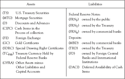
Exhibit 4.4 Combined Balance Sheet for Federal Reserve Banks

Equation 4.9 is the base money equation for the U.S.² Nearly all the entries are from the Federal Reserve balance sheet. Because base money is either used as bank reserves (R) or circulating currency (C), the sum of R and C is known as the uses of base money. Total bank reserves (R) are viewed as the Federal Reserve defines them: total commercial bank balances at Federal Reserve Banks (MBD) plus total bank vault cash (BVC). Bank vault cash consists of currency holdings by commercial banks. It is in the form of coins issued by the U.S. Treasury (TC_B) and paper notes issued by Federal Reserve banks (FRN_B).

Currency in circulation (C) is total currency circulating outside of banks. It consists of Treasury-issued coins owned by the public (TC_P) and Federal Reserve Notes owned by the public (FRN_P). When an individual goes to the bank (or a teller machine) and withdraws currency, the level of the monetary base remains unchanged but the uses of the monetary base have changed. C (in the form of FRNp) increases and R (FRN_B, a component of bank vault cash) falls. If an individual deposits currency, it, likewise, has no effect on the level of base money. The composition of base money, however, again changes.

All variables to the right of the identity sign (starting with TS) are sources of the monetary base. They include both factors of increase and factors of decrease. Those with a positive sign (TS, MTG, D, F, G,...) are factors of increase. If they increase (decrease), and the offsetting accounting entry in equation 4.9 is B, then the monetary base increases (decreases) on a one-to-one basis. Variables with a negative sign (TCH, TRD, FD) are factors of decrease. If they increase (decrease), and the offsetting accounting entry in the base money equation is B, the monetary base decreases (increases). The relationship is one-to-one, but inverse.

Federal Reserve Float (F)

The first four terms on the right-hand side of the base money equation (TS, MTG, D, and F) all originate in the Fed’s balance sheet, and each is a factor of increase. Collectively (TS + MTG + D + F), they are called Federal Reserve Credit. This measures the quantity of base money that exists as a consequence of Federal Reserve actions. U.S. Treasury security holdings by Reserve Banks (TS), total mortgage securities owned by the Federal Reserve (MTG), and total commercial bank borrowings at the Federal Reserve Bank discount window (D) are the result of monetary policy and are discussed in the following sections.

The fourth, Federal Reserve float (F) is not due to monetary policy, but relates to the Federal Reserve procedures for clearing checks. It is calculated as the net of two items in the Federal Reserve balance sheet. Federal Reserve Float is equal to cash items in the process of collection (CIPC) minus deferred availability of cash items (DACI). That is, F = CIPC - DACI.

CIPC is a Federal Reserve asset, and records the volume of cash items in the form of checks that the Fed owns. Banks sent these checks to the Federal Reserve for clearing purposes. How the Federal Reserve pays for these checks is also recorded in the Fed’s balance sheet. A few cash items receive immediate (or same day) credit, and the offsetting entry is a liability item in the Federal Reserve balance sheet: MBD. The bank submitting this cash item is credited with bank reserves in the form of a larger checking account balance at the Federal Reserve Bank.

While all banks eventually receive reserves (MBD) for checks they send to the Fed, they do not receive immediate reserve credit for most cash items. Instead, the Federal Reserve schedules to pay them reserves at a later date. According to the Fed’s processing procedures, reserve payment will occur either one day or two days later. Timing of the payment is based on a predetermined geographic grid as well as the type of cash item submitted. That scheduled payment is entered in the balance sheet as liability item: deferred availability of cash items (DACI).

Note that the Federal Reserve’s procedures for giving reserve credit to banks submitting cash items is not determined by when they collect on these checks. Consequently, their clearing procedures have monetary implications. The Federal Reserve often credits a bank (that sent a cash item) with reserves prior to collecting on the check. When that happens, total reserves in the banking system increase. Federal Reserve float is a measure of the total quantity of reserves in the banking system that entered in this manner. The volume of float varies from day-to-day and is influenced by factors such as weather conditions and the geographic features of market sales. Local purchases are less likely to result in Federal Reserve float than are national or international purchases.

An example of Federal Reserve float is shown in Exhibit 4.5. In transaction 1), Bank A sends a check to the Federal Reserve Bank. The offsetting entry in the bank’s balance sheet is DACI (+), a scheduled payment of bank reserves by the Fed. In the Fed’s balance sheet, both CIPC and DACI increase by the same amount. Hence, total Federal Reserve float is unchanged.

Exhibit 4.5 Federal Reserve Float

Assume that two days pass, and the Federal Reserve credits Bank A with reserves (MBD_A +) even though it has yet to collect on the check. This is transaction 2). If one combines transactions 1) and 2), the Federal Reserve balance sheet shows that CIPC is up, but DACI is not. Federal Reserve float increased with the second transaction.

The Fed will eventually collect on this check and when they do, they will reduce the reserves of the Bank B (MBD_B −), the bank upon which the check is drawn. This check will have effectively cleared the system, and there is no longer any float associated with that instrument. The increase in reserves at Bank A is exactly offset by a drop in reserves at Bank B. These entries are shown as transaction 3) in Exhibit 4.5.

Treasury Deposits (TRD)

Treasury deposits at Federal Reserve Banks (TRD) are also a variable in the base money equation. The U.S. Treasury uses Federal Reserve Banks for banking purposes. It owns deposit balances at Reserve banks, and writes checks on those balances in order to make payments. Those deposit balances are referred to as Treasury deposits (TRD), and appear as a liability item on the combined balance sheet for Federal Reserve Banks.

This item in the Fed’s balance sheet (TRD) also appears as a factor of decrease in the base money equation 4.9. When the Treasury writes a check on its account, the check ultimately clears the banking system. The commercial bank submitting the check to the Federal Reserve receives deposit credit at a Federal Reserve Bank. Thus, bank reserves (and base money, B) increase, but TRD falls when the Federal Reserve Bank cancels the check the Treasury wrote to make the payment. The opposite happens when someone sends a check to the Treasury and the Treasury deposits that check at a Reserve Bank. TRD increases and MBD decreases.

Consider an example where individual A, who banks at Bank A, makes a tax payment to the Treasury. Payment by individual A is in the form of a check drawn on Bank A. The T-accounts for this transaction are in Exhibit 4.6. Only final entries in the T-accounts are shown, i.e., intermediate transactions such as the deposit and the clearing of the check do not appear.

Exhibit 4.6 Individual Tax Payment to the Treasury

Having written a check to pay his taxes, individual A now has a lower checking account balance (DD√ −). The offsetting balance sheet entry is a decline in his net worth (NW). That occurs because the tax payment is not a quid pro quo transaction. The tax payment is compulsory with no specific goods or services received in exchange.

The balance sheet for Bank A shows individual A’s lower deposit balance. This is offset by Bank A’s lower deposit balance at the Federal Reserve Bank (MBD −). The Treasury deposited individual A’s check at the Federal Reserve Bank. When the Fed sent that check back to Bank A (for clearing purposes), it lowered Bank A’s deposit balance as payment for the check.

The Treasury now has a larger cash balance at the Federal Reserve Bank (TRD +), with the offsetting entry an increase in its new worth (NW +). With its higher cash balances, the Treasury is now in a position to purchase more goods and services. As a consequence of paying taxes, the private sector (individual A) is in a position to purchase fewer.

From a monetary standpoint, base money is lower. That is because TRD is a factor of decrease in the base money equation. The reduction in base money appears in T-accounts as a decline in MBD. These deposits are a component of bank reserves. Thus, in equation 4.9, B (in the form of R) is lower, while TRD is higher.

Treasury management of its cash position, then, affects the quantity of base money. Hence, Treasury actions can potentially impair the effectiveness of monetary policy. For that reason, there is daily communication between the Treasury and the Federal Reserve concerning Treasury budgetary activity for that day. This allows the central bank an opportunity to take actions that offset the monetary repercussions of Treasury fiscal actions.

The (Base) Money Multiplier

In a world of fiat money with fractional reserve banking, the money multiplier is greater than one. This means that whenever the level of base money changes, the money supply changes by some multiple of that change in the base. The extent of the change in money supply depends on the size of the base money multipler (m). The M1-multiplier is presented as equation 4.10. There are three factors that determine the size of m: k, r_r, and r_e³

where k is the currency ratio,

r_r is the average reserve ratio requirement, and

r_e is the excess reserve ratio.

where C is total currency in circulation outside banks, and DD√ is total checkable deposits.

where RR is total required reserves for banking institutions.

where ER is total excess reserves held by banks.

The Currency Ratio: k

The currency ratio (equation 4.11) is a behavioral ratio, whose value is determined by the general public. It measures how much currency the public chooses to hold relative to their holdings of checkable deposits. k is also an aggregate ratio, i.e., the value of k is an average ratio for the entire public.

Because k appears in both the numerator and denominator of the money multiplier, it is not immediately clear whether the relationship between m and k is direct or inverse. If k increases, both the numerator and denominator of m increase. Similarly, a decline in k results in a lower value for both the numerator and denominator.

While the mathematics is not developed here, for reasonable values for the other parameters in m, the relationship between m and k is inverse (∂m / ∂k < 0.) The change in m divided by the change in k is less than zero. Increases in the currency ratio cause the money multiplier to fall; decreases cause it to rise.

The reason for this inverse relationship becomes apparent by examining equations 4.14 and 4.15. It has to do with how the monetary base is used. Every unit of base money that is held as circulating currency (C) maps into exactly one unit of money (M1). The relationship is one-to-one. On the other hand, every unit of base money that is used as bank reserves (R) maps to some multiple of that value in terms of deposit money (DD√). That relationship is one-to-x, where x > 1.

Thus, base money supports a larger money supply when it is used as bank reserves. The reason is fractional reserve banking (R < DD√). When individuals deposit their currency in banks, that currency becomes bank reserves (R ↑ and C ↓). These bank reserves support some multiple level of deposit money in a world of fractional reserve banking. Had the individuals continued using the currency instead of depositing it, there would be no such multiple impact on the money supply.

When the currency ratio (k) changes so too, does the base money multiplier (m). Consequently the portfolio behavior of the general public has monetary significance. Decisions concerning how much currency to hold relative to deposit money influence the level of the money supply through changes in the money multiplier.

There are seasonal, cyclical, and secular influences on the public’s portfolio behavior (and, thus, k). An important seasonal influence is the Christmas holiday season in the United States. Related to the sharp acceleration in December retail sales is a greater demand for currency to effectuate those sales. The higher currency ratio has a depressive influence on the money multiplier and the money stock. That upward blip in the currency-ratio generally is reversed in January, when retail sales most often fall.

One of the more dramatic movements in the currency-ratio occurred during the Great Depression in the 1930s. The public lost confidence in commercial banks and many chose to hold their money in the form of currency rather than bank deposits. This led to a sharp decline in the money multiplier, which contributed significantly to a massive decline in the money supply.

Another factor affecting the currency ratio is the process of economic development. The ratio tends to fall with economic growth as financial institutions and markets develop. The public typically reduces its reliance on currency, and more frequently makes payment with deposit money. One hundred years ago, it was not uncommon for U.S. workers to receive their wages in the form of currency. That rarely occurs today. Most individuals receive payment either by check or via direct deposit.

The Reserve Ratio Requirement: r_r

Banking is a very highly regulated industry. That is true even in those countries where most markets are open, and voluntary exchange generally is permitted. One form of banking regulation is reserve requirements. This regulation requires banks to hold reserves in a specified minimum ratio to their deposit liabilities.

While it is possible to have reserve requirements for several categories of bank deposits, only the reserve requirement on checkable deposits (r_r) is considered here. If r_r = 10%, for example, banks are required to hold reserves in the proportion of at least 10% of their checkable deposit liabilities. Equation 4.16 shows the calculation for required reserves (RR). If r_r = 10%, and total DD√ is equal to one million dollars, RR = $100,000.

The reserve ratio requirement is in the denominator of the money multiplier. This indicates an inverse relationship between r_r and m. A higher reserve ratio requirement means a lower money multiplier. A lower money multiplier, in turn, results in a lower money supply. A lower reserve ratio requirement, by contrast, leads to monetary expansion.

The inverse relationship between r_r and m exists because reserve requirements restrict the amount of lending (and money creation) banks can potentially undertake. However, recent changes in the reserve ratio requirements for U.S. banks indicate that, for this country, r_r is less of a constraint on bank lending than it was in the past. These changes in U.S. reserve requirements, and their implications for the U.S. money multiplier, are described in Section C.

Excess Reserve Ratio: r_e

Reserve requirements specify legal minimum proportions of reserves to deposits. Banks are free to hold additional reserves, and often have. These additional reserves are called excess reserves. In equation 4.17, the volume of excess reserves (ER) is calculated as the difference between total reserves (R) and required reserves (RR).

Excess reserves are low-earning assets and holding them generally reduces bank profits.⁴ Hence, banks must have an overriding motive if they are to hold any excess reserves. When they do so, it is generally because of uncertainties surrounding the management of their cash position. These problems relate to difficulties associated with forecasting deposit withdrawals and loan demand.

Banks do not know, with certainty, the amount of deposit withdrawals and loan demand that will occur on any given day. Both of these activities result in a reduction of a bank’s reserve position. Consequently, banks must have a strategy for coping with these uncertainties. One such strategy is called asset management. This involves holding liquid assets in the bank portfolio. When pressures on the cash position do occur, these liquid assets can be sold. Because excess reserves are the most liquid of assets, they sometimes are held for this purpose.

When banks hold excess reserves, those reserves are not available to support bank lending activity. From the perspective of bank lending (and the accompanying money creation), it is as if the reserves do not exist. That is, the holding of excess reserves reduces the potential size of the money supply.

It does so through the money multiplier. The excess reserve ratio (r_e) is in the denominator of the multiplier, indicating an inverse relationship. As banks hold more excess reserves, in relation to their checkable deposits (r ↑), the money multiplier is smaller. A smaller value for m implies a reduction in M1. Reducing excess reserve holdings (relative to DD√), on the other hand, expands the money supply.

A Numeric Example

The general public, commercial banks, and the government potentially influence the size of the money stock through the money multiplier, whose value depends on the levels of k, r_r, and r_e. k is determined by the behavior of the general public; r_e, by the behavior of commercial banks. Given the practice of bank sweeps in the United States (pp. 85−87), r_r is also largely determined by commercial banks. That is the case even though stated reserve requirements originate through government.

Other things equal, all three are in an inverse relation to m. Assume, for example, that k = .5, r_r = .05, and r_e = .05.

From equation 4.2, a multiplier of 2.5 indicates that the money supply is 2.5 times the level of the monetary base. Moreover, from equation 4.3, any change in the level of the monetary base results in a change in the money supply that is 2.5 times the change in the quantity of base money. This multiplier effect, which is the direct consequence of fractional reserve banking, has very important consequences for monetary policy. If bank reserves are increased through monetary policy, there will be a multiple expansion of bank deposits. A reduction in reserves leads to a multiple contraction of bank deposits. This phenomenon is known as the multiple expansion and contraction of bank credit.

General Instruments of Monetary Control

There are four general instruments of monetary policy: 1) open market operations; 2) discount window/discount rate; 3) reserve ratio requirements; and 4) interest payments on bank reserves. They are called general instruments because their effects are widespread. That is, their usage has an impact throughout the country, and across most markets. This has important political implications, especially for democracies. In situations where monetary policy inflicts economic hardship, it is more politically palatable (or considered a “fair game”) if it affects nearly everyone.

Open Market Operations

History

Open market operations are the purchase and sale of securities by the central bank. They are by far the most important monetary-policy instrument in the United States today. This was not always the case. Indeed, when the Federal Reserve Act was passed in 1913, there was no understanding of this instrument. The Act did empower individual Reserve banks to purchase U.S. government securities and bankers acceptances. The motives were twofold: 1) to allow Reserve Banks to earn additional income to cover operating expenses; and, 2) to promote international trade.

The potential impact of such purchases (and sales) on economic activity was discovered by accident in the early 1920s. This discovery led to the formation of a series of committees within the Federal Reserve System. The motive was to coordinate security purchases and sales by individual banks. If open market purchases and sales did significantly affect the economy, an attempt to coordinate these actions made sense.

Ultimately, open market purchases and sales were codified into law with the Banking Acts of 1933 and 1935. The 1933 legislation provided for a Federal Open Market Committee (FOMC) that would assume responsibility for the conduct of open market operations. No longer were individual Banks allowed to purchase and sell securities. Instead, purchases and sales were done on behalf of all 12 Federal Reserve Banks. Individual Banks could refrain from participation, but that option was removed in the Banking Act of 1935.

The Process

Open market operations originate with the FOMC, which meets approximately every six weeks. Intra-meeting decisions occasionally occur via conference call, but they are the exception. FOMC meetings include both the presentation of economic forecasts and policy discussion. They end with the issuance of a set of instructions (called a directive) to the Account Manager of the Federal Reserve Bank of New York. The directive is written in general terms, but the Account Manager is in attendance at the meetings to capture the intent of the FOMC committee. The Account Manager then uses the directive to carry out open market operations on behalf of all twelve Reserve Banks.

Federal Reserve purchases and sales of securities occur via a process known as the “go around.” Once the Account Manager decides a course of action, he/she informs traders at the New York Federal Reserve Bank. These traders, in turn, contact security dealer firms in the New York City money market. Actual trades are between the New York Fed and these dealer firms.

Assume, for example, that the Account Manager’s decision is to buy a given quantity of U.S. government securities within a specific maturity range. Traders contact individuals at the security dealer firms and ask them if they have any such securities for sale. If they do, traders want to know how many and at what price? Dealer firms offering securities are asked if they are willing to hold firm on their offers for the next 30 minutes. All offers are posted at the New York Fed, and the decision is made to accept or reject the offers. Typically, the Fed buys securities with the lowest offer price (and the highest yield). Once the decision is made, traders again contact the security firms and inform them if their offers are accepted or rejected.

Most U.S. open market operations involve secondary-market purchases or sales of U.S. government securities. Even though U.S. Treasury securities are exchanged, the U.S. Treasury (who issued the securities) is not involved. The Treasury issued these securities at some time in the past, and someone else owns them now.

The fact that open market operations are conducted in the secondary market for U.S. government securities has an important implication. They do not affect the overall size of U.S. government debt. What changes is the composition of ownership of U.S. Treasury debt. If the Fed purchases securities, more of the debt is now owned by Federal Reserve Banks, and less is owned by security dealer firms.

Accounting for Open Market Operations

The monetary impact of open market operations is determined by how the transactions are financed. Purchases and sales by the Federal Reserve are paid with bank reserves. Payment is made on a pass-through basis, and involves the Fed, a set of security dealer firms, and the clearing banks for the dealer firms.

The T-accounts associated with an open market purchase are presented in Exhibit 4.7. As a simplification, it is assumed that only one security dealer firm (Firm D) and one clearing bank (Bank D) are involved. The combined balance sheet for Federal Reserve Banks shows an increase in Treasury securities (TS) on the asset side. This records the acquisition of securities.

Exhibit 4.7 T-Accounts for Open Market Purchase

The offsetting entry is an increase in MBD on the right-hand (liability) side. MBD is total commercial bank deposits at Federal Reserve Banks. The increase in this item on the Fed’s balance sheet indicates how the Federal Reserve paid for securities acquired in the open market purchase. The Fed does not directly pay the security dealer firm (Firm D) but, instead, pays the clearing bank (Bank D) for the security dealer firm. It does so by increasing that bank’s deposit balance at the Fed. Bank D then passes the payment through to dealer firm.

The pass-through payment is shown on the T-account for Bank D. This clearing bank now has a larger deposit balance at the Federal Reserve Bank, but also has an increase in its deposit liabilities (DD√). This increased checking account balance is owned by the security dealer firm (Firm D), and represents the pass-through payment from the clearing bank to Firm D. The T-account for Firm D now shows both the increase in its deposit balance at Bank D and a reduction in its holdings of U.S. government securities.

Open Market Operations and the Money Supply

Commercial bank balances at Reserve Banks (or member bank deposits, MBD) count as bank reserves. When the Federal Reserve pays for securities by increasing these balances, the total volume of reserves in the banking system increases. Because banks need reserves in order to make loans, banks are now in a position to extend more credit.

This has important implications for the money supply. When banks make additional loans, the money supply increases. Indeed, in a world of fractional reserve banking, there will be a multiple expansion of bank credit. In the above example, the raw material for such a multiple expansion of bank deposit money appears in the form of additional bank reserves at Bank D.

The world of fiat money is a world of inflation, and this secular decline in the purchasing power of money largely is the consequence of government expansion of the money supply. For many market-oriented economies in the industrial world, expansion the money supply occurs mainly through such open market purchases. In these economies, open market operations now serve as the “printing press.”

Open market purchases (and sales) of securities affect the base money equation 4.9. Federal Reserve purchases increase TS (a factor of increase), with the offsetting entry an increase in base money (B). In the basic money supply model (4.2), the increase in B results in an increase in M1. The multiple expansion of deposit money occurs through the workings of the money multiplier, which is larger than one in a world of fiat money and fractional reserve banking. The impact of those changes on equation 4.2) is shown below.

Transmission of Bank Reserves

In this country, new reserves brought into the system via open market purchases are initially located in New York City banks. That is because open market operations are with dealer firms and clearing banks in New York City. Some of the new reserves may be used to support lending activity in this locale. However, reserves tend to follow economic activity and the newly created reserves can be used to support lending activity in any part of the country. Avenues for the transfer of these reserves from Bank D to other parts of the country (or world) are many. Only a few are mentioned here.

One possibility is that a New York City firm borrows money from Bank D and spends the proceeds of the loan outside the city. Another is that a firm outside New York City borrows from Bank D and, likewise, spends the funds outside of New York City. Still another possibility is that the reserves will leave New York City through activity in the federal funds market. This last possibility is examined in more detail.

The federal funds market is one where immediately available (or same day) funds are loaned. These funds must be immediately available because many of the loans are for one day only. This market has long been a medium for the transfer of bank reserves. Activity in the market commenced in the early 1920s, with banks loaning reserves to one another on an overnight basis. The market flourished during the final third of 20th century, with many small banks joining the ranks of large banks by using the market as a medium for adjusting their short-term reserve positions. Some of the more aggressive larger banks commenced to use the market for more than simply adjusting their reserve position. The reserves they acquire are employed to support their long-term loan portfolios.

Exhibit 4.8 shows T-accounts for a typical federal-funds market transaction. In this example, Bank D loans reserves to Bank DBQ in Dubuque, Iowa. Bank D instructs the Federal Reserve to transfer a portion of its reserves to the account of Bank DBQ. When this happens, there is no change in the aggregate volume of commercial bank balances at Federal Reserve Banks. However, there is a change in the ownership composition of these balances. The Fed’s balance sheet shows an increase in MBD_DBQ (Bank DBQ’s balance) and a decrease MBD_D (Bank D’s balance).

Exhibit 4.8 Federal Funds Market Transaction

Bank D has swapped assets. Its balance sheet shows an increase in federal funds sold (FFS +) and a decrease in its reserve balance at the Fed (MBD_D−). The balance sheet for Bank DBQ reflects its larger reserve balance at the Fed (MBD_DBQ +), and an increased liability for federal funds purchased (FFP +). The bank reserves created by the New York Federal Reserve Bank’s open market purchase now reside with Bank DBQ in Dubuque, Iowa.

Discount Rate/Discount Window

A second general instrument of monetary policy is the discount rate. This is the interest rate the Federal Reserve Bank charges banking institutions when they borrow reserves at the discount window. When the Federal Reserve System was initially organized in 1914, the country was still operating with fiduciary money (the gold standard). At that time, the discount rate was the principal instrument of monetary control. The United States was following in the footsteps of the United Kingdom, where the bank rate of Bank of England had long been the centerpiece of monetary policy. But, there was more to it than that. Open market operations were not understood in 1914, and reserve ratio requirements were set by statute. Hence, the discount rate was the only general instrument of monetary control.

Individual Reserve Banks set the discount rate with the approval of the Federal Reserve Board. There were many instances, early in the history of the Federal Reserve System, when the discount rate was not uniform across all Federal Reserve Districts. That is uncommon today, where a uniform discount rate policy across Federal Reserve Districts reflects the high degree of integration of financial markets in the United States.

For decades, the Federal Reserve employed nonprice rationing in managing the discount window. This was due, in part, to prolonged periods where the discount rate was set below the federal funds rate. To limit bank borrowing through the discount window, the Fed established rules and guidelines for appropriate commercial bank use of the discount window. These rules and regulations were known as the Federal Reserve’s “administration” of the discount window. The Fed made it known that banks should use the discount window mainly as a means of managing their short-term reserve position. Continuous borrowing was frowned upon and considered a violation of Fed policy.

The Federal Reserve recently changed its discount window policy. Regulation A was revised in a manner that eliminated much of the nonprice rationing at the discount window. The Fed increased the discount rate by 150 basis points, and placed it 100 basis points above the federal funds rate. All banks in sound condition, and with adequate collateral, now are permitted discount-window borrowing at their own discretion. With the discount rate above the federal funds rate, banks generally have an incentive to adjust their reserve positions in the federal funds market.⁵

During the first two decades of the Federal Reserve System, the discount window was a major source of bank reserves and of variation in the monetary base. The proportion of reserves coming through the discount window did not fall below 37% in the 1920s, and was in excess of 80% in 1921. During this period, changes in the discount rate were of major significance. That is no longer the case. With the ascendance of open market operations as the primary instrument of policy, the importance of the discount window has steadily diminished.

In recent decades, the ratio of borrowings at the discount window to total bank reserves was often is less than 1%. This indicates that virtually none of the bank reserves were coming through the discount window. Although this is an overstatement, current changes in the discount rate are tantamount to a price change in a market where there is no activity.

While the significance of the discount rate has diminished, officials of the Federal Reserve are not ready to abolish the discount window. It can play a major role when the Fed assumes the posture of lender of last resort. The central bank plays that role in situations that could result in financial panic. Three recent incidents were the stock market crash in 1987, the terrorist attacks on the New York City Twin Towers in 2001, and during the Great Recession of 2008−2009. During such episodes, the Federal Reserve often is desirous of making sizable volumes of bank reserves available on short notice. The discount window is well suited for this purpose.

Both open market purchases and lending through the discount window provide additional reserves to the banking system. From a policy perspective, however, they differ in one critical respect. In the case of open market purchases, the Federal Reserve takes the initiative. For loans through the discount window, individual commercial banks must initiate activity. That is, nothing happens until a bank approaches the Fed and requests a loan.

T-Accounts for a discount window loan appear in Exhibit 4.9. Bank A requests and receives a loan from a Federal Reserve Bank. The loan appears in the Fed’s balance sheet as an increase in D (Discounts and Advances). The proceeds of the loan are made available to Bank A in the form of an increased deposit balance at the Federal Reserve Bank. Hence, MBD_A increases on the right-hand side of the Fed’s balance sheet.

Exhibit 4.9 Discount Window Loan

Bank A owns that deposit balance, which shows as a left-hand side entry in its balance sheet (MBD_A +). The offsetting entry is on the liability side (D +). This additional liability reflects Bank A’s obligation to repay that loan at a later date.

Discounts and Advances (D), from the Fed’s balance sheet, are a factor of increase in the Base Money Equation 4.9. Hence, a discount-window loan increases the level of monetary base. Repayment of the loan has the opposite effect. It decreases the monetary base. The affect that increased lending through the discount window has on the money supply is seen in equation 4.20 below. Again, with fractional reserve banking, an increase in base money results in a multiple expansion of deposit money.

Reserve Ratio Requirements

Banking started as individual proprietorships or partnerships that were unregulated. Today, most banks are corporations that are very heavily regulated by government. Reserve requirements are one form of government regulation. These regulations specify that commercial banks must hold reserves in some minimum proportion to bank deposit liabilities.

When the Federal Reserve Act was passed in 1913, reserve requirements were set by statute. The Banking Act of 1935 gave the Federal Reserve Board the authority to set (and change) reserve requirements for all federally chartered banks. The Depository Institution Deregulation and Monetary Control Act of 1980 extended the Federal Reserve’s authority to cover all depository institutions—both bank and nonbank institutions, and state chartered as well as federally chartered depository institutions.

Unlike open market operations and lending through the discount window, changes in reserve requirements do not affect the total volume of reserves in the banking system. Instead, changes in reserve requirements affect the maximum amount of deposits a given volume of reserves will support. When reserve requirements are increased, available bank reserves potentially support a smaller quantity of bank deposits. A decrease in reserve requirements has the opposite effect. Available reserves can now support a larger quantity of bank deposits.

Bank A in Exhibit 4.10 below has $100,000 in deposits. With a 10% reserve requirement, its required reserves are $10,000. Because Bank A has exactly that amount of reserves, it is holding zero excess reserves. In banking parlance, the bank is “loaned out.”

Exhibit 4.10 Balance Sheet – Bank A

If the central bank lowers the reserve requirement to 5%, the total quantity of reserves in the banking system is not affected. That is true for Bank A as well, which still has $10,000 in reserves. However, its required reserves have fallen to $5,000. With excess reserves in the amount of $5,000, it is now in a position to make additional loans. Doing so will expand the total quantity of deposit money.

Were the central bank to, instead, increase the reserve requirement, the opposite occurs. While Bank A’s reserves remain the same, it now has a deficient reserve position, or negative excess reserves. It must now make fewer loans which contracts the total quantity of deposit money.⁶

Such changes in reserve requirements have their monetary impact through the money multiplier. As discussed in pages 73–74, the reserve requirement is in the denominator of the money multiplier. Hence, the size of the multiplier moves inversely with the level of the reserve requirement. For example, a reduction in the reserve requirement increases the size of the multiplier, as in equation 4.21 below.

Changes in reserve requirements have been infrequently used as a means of adjusting monetary policy. For that reason, they have been a minor instrument of monetary policy. Recently, many banks in the United States commenced new banking practices (with sanction from the Federal Reserve) that further diminished the significance of reserve requirements.

Beginning in 1994, these commercial banks began to reclassify a portion of their checkable deposits liabilities as money market deposit accounts (MMDAs). Such reclassifications, referred to as sweeps, were motivated by the desire to limit the impact of reserve ratio requirements.⁷ Because they were done only for reserve accounting purposes, sweeps did not alter the nature of the securities owned by bank customers. However, banks employing sweeps now had two sets of books (or balance sheets). One set was for reserve accounting; the other, for general dissemination.

Use of sweeps effectively lowered a bank’s reserve requirements. The reason is that checkable deposits were subject to reserve requirements, while MMDAs were not.⁸ By reducing the bank’s level of checkable deposits (for reserve accounting purposes), sweeps had the effect of reducing a banks required reserve holdings. The same level of checkable deposits now called for fewer required reserves. Banks using these sweeps had, in effect, lowered their own required reserve ratio. The bank’s new required reserve ratio was below the one specified by the Federal Reserve.

Following is a summary of the critical features of these new reserve ratio requirements:

Given the implications for monetary policy, the last feature requires elaboration. Following sweeps, the new lower reserve requirement is not a binding constraint for many banks. The reserves they choose to hold to meet customer demands for credit, and for potential adverse check clearings, are above the level of required reserves. For banks in such a position, an increase or decrease in the Federal Reserve’s reserve requirements is likely to leave them in a similar position. That is, their required reserves are still below those they choose to hold for normal banking operations. As a consequence, the change in the Fed’s reserve requirements may have no impact on the bank’s level of desired reserve holdings and lending policies.

With reserve requirements for many banks below those specified by the Fed, and with the Federal Reserve’s reserve requirements having only a negligible impact on many banks, an alternative version of the base money multiplier is presented. In contrast to the multiplier in equation 4.10, it focuses attention on total reserve holdings of banks instead of partitioning them into required and excess reserves.

Let r = r_r + r_e, where r is an aggregate reserve ratio for banks. Given the Federal Reserve’s diminished role in establishing reserve requirements, r is largely determined by commercial bank behavior. With the currency ratio (k) determined by the behavior of the general public, the size of the reconstituted money multiplier (equation 4.22) is largely determined by the behavior of economic agents in the private sector.

Interest on Bank Reserves

In 2008, the Federal Reserve began paying interest on commercial bank deposits at Federal Reserve Banks (MBD). Prior to this time the Federal Reserve paid no interest on these deposits. Because MBD are a component of the cash position of a commercial bank, this change in Federal Reserve policy increases the income banks earn by holding this form of cash.

Payment of interest on MBD (i_MBD) also gives the Federal Reserve a new policy instrument. By varying the interest paid on these deposits, the Federal Reserve can influence the desired level of excess reserve holdings by commercial banks. Because excess reserves are reserves not employed to support bank lending, changes in the level of excess reserve holdings by banks influences both the volume of bank lending and the level of the money supply.

An increase in i_MBD increases commercial bank returns on excess reserves. They now have an incentive to make fewer loans and to hold more excess reserves. If they do so, the money supply decreases. A reduction in i_MBD has the opposite effect. It reduces the incentive for banks to hold excess reserves. If banks respond by making additional loans, the money supply increases.

Thus, Federal Reserve changes in i_MBD have their impact on the money supply through the base money multiplier. The aggregate excess reserve ratio for commercial banks (r_e) is now a function of the rate the Fed pays on deposits that banks hold at Federal Reserve banks, or i_MBD. The revised version of the multiplier is shown in equation 4.23. A higher level of i_MBD increases r_e and reduces the level of base money multiplier; a lower level of i_MBD does the opposite. It lowers r_e and increases the money multiplier.

Selective Credit Controls

When a central bank directs credit to specific markets, specific firms, or specific regions of the country, this is known as selective credit controls. This practice is common in socialist countries and/or less developed countries where governments often desire greater control over how resources are employed in the economy. In a socialist country, for example, the government may want to increase the size of the manufacturing sector of the economy. If the central bank channels more credit to this sector of the economy, it can increase the prospects for greater economic activity in manufacturing.

In the U.S. recession of 2008–2009, the Federal Reserve deviated from it historical pattern of relying on general instruments of monetary control. Instead, it moved into the realm of selective credit controls. It did so through the direct placement of bank reserves, both in specific banks and in a specific sector of the U.S. economy.

Purchase of Bank Equity (BKEQ)

The Federal Reserve coerced the largest U.S. banks to sell bank equity to the Fed. The motive was to increase the capital position of those banks. The Federal Reserve was concerned about the capital adequacy of these banks once they wrote down the value of their assets to reflect the reduced quality of their loan portfolios.

Some interpreted this as an attempt by the U.S. government to socialize banks in the country. This partly reflected the unprecedented nature of this action. But, it also reflected a legitimate concern. At issue was whether the government would eventually become a major shareholder in these banks. If that were to occur, banks would be effectively socialized. Moreover, the government would be in a position to engage in selective credit controls on a continuing basis.

The immediate consequence of the Fed’s actions was to increase the capital position of the banks involved. It did so by directly placing bank reserves in those banks in exchange for bank equity. The impact on balance sheets is shown in Exhibit 4.11. The Federal Reserve now holds bank equity (BKEQ +) on the asset side of its balance sheet. This purchase of commercial bank stock was financed by increasing its liabilities in the form of a larger deposit balance for the bank selling equity to the Fed.

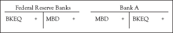
Exhibit 4.11 Federal Reserve Purchase of Bank Equity

This new deposit balance (MBD +) is an asset for the selling bank, Bank A, and appears on the left-hand side of its balance sheet. The offsetting entry for Bank A is an increase in bank equity (BKEQ +). The higher level of Bank A’s equity represents an increase in the capital position of the bank. A similar increase bank capital occurs for each bank selling its equity to the Federal Reserve.

While the Federal Reserve’s motivation was to increase bank capital for individual banks, these actions also have monetary implications. Because the Fed paid for its new bank equity holdings with bank reserves, base money increases. In the equation for base money, 4.9, BKEQ is a component of Other Federal Reserve Accounts (OFRA). When this factor of increase rises so too, does the monetary base. With additional reserves (MBD +), banks are now in a position to make more loans and create additional deposit money.

Purchase of Mortgage Securities (MTG)

The Federal Reserve also engaged in selective credit controls when it directly placed reserves with individual commercial banks in exchange for mortgage securities during the Great Recession of 2008–2009. Through such exchanges, the Fed was directly channeling credit to a specific sector of the U.S. economy—the housing sector. The motive was to provide financial support for that sector which was at the epicenter of the very pronounced decline in economic activity.

When the Federal Reserve purchased mortgage securities from banks, it not only provided direct support to the housing sector, but also support for individual commercial banks. The mortgages sold by these banks were often “nonperforming,” i.e., the borrower was in arrears on equity payments, interest payments, or both. Selling these toxic assets to the Federal Reserve enabled many of these banks to avoid severe financial stress and, for some, the prospect of bankruptcy. From the perspective of the Federal Reserve, shoring up individual bank balance sheets in this manner reduced the possibility of contagion, where the failure of one bank can lead to the failure of many banks, and possibly resulting in a general financial panic.

The impact of Federal Reserve purchases of toxic mortgage securities from individual commercial banks is shown in Exhibit 4.12. The Federal Reserve now owns mortgage securities which it financed by crediting the account of the selling bank, Bank A, with a deposit at the Federal Reserve Bank. Bank A shows that new deposit balance as an asset (MBD +) on the left-hand side of its balance sheet. The offsetting entry is a drop in its holdings of mortgage securities (MTG –).

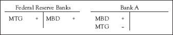
Exhibit 4.12 Federal Reserve Purchase of Mortgage Securities

The Federal Reserve’s payment for these securities was in the form of new bank reserves. In the base money equation 4.9, MTG increases as does B. The banking system, in general, is now in a position to extend additional credit. The Federal Reserve provided a massive amount of bank reserves to the financial system in this manner during and after the recession of 2008–2009. From a position of zero holdings prior to 2008, MTG became one of the larger assets in the Federal Reserve’s portfolio.

BKEQ and MTG are both on the asset side of the combined balance sheet for Federal Reserve Banks, and are factors of increase in the base money equation. Hence, both the purchase of bank equity and the purchase of mortgage securities by the Federal Reserve increase the quantity of base money and, potentially, the money supply. Those changes are summarized in equation 4.24. The sale of these securities has the opposite effect. It decreases the quantity of base money and the money supply.

Closed Market Operations

From a global perspective, most money creation is not based on the policy instruments discussed above. The largest share of the world’s fiat money is created in less developed countries and/or countries that have embraced socialism.

Open market operations are often not an option for these countries because financial markets are so poorly developed.⁹ Poorly developed markets, however, have not hampered their ability to create fiat money. Money supply increases in these countries are often the result of a process referred to here as closed market operations.

Monetary policy generally is driven by government financing operations. Governments wish to spend more money than the Treasury obtains in tax revenues. With no active market for Treasury securities, the government cannot finance additional spending by selling Treasury bonds in the open market. Instead, the Treasury issues new bonds and places them directly with the central bank. The central bank pays for these securities by crediting the deposit account of the Treasury at the central bank. The Treasury now is in a position to spend more.

The T-accounts for this closed market operation are in Exhibit 4.13. The Treasury balance sheet shows an increase in its cash balance at the central bank (TRD +). The increase in Treasury liabilities (TS +) represents the bonds (or Treasury Securities) placed directly with the central bank. The balance sheet for the central bank shows that this institution now owns more Treasury securities (TS +). The offsetting entry is the increase in the Treasury’s deposit balance (TRD +) with the central bank.

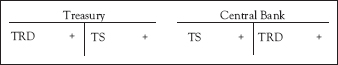
Exhibit 4.13 Closed Market Operations

Once the Treasury spends these new cash balances, Treasury deposits at the central bank (TRD) are transformed into bank reserves (MBD). Banks are now in a position to extend additional credit. Massive amounts of fiat money are created in this fashion.

APPENDIX A

Derivation of the Base Money Equation

The base money equation is an accounting identity. It is derived from two other identities: 1) the balance sheet for the central bank; and 2), the Treasury Monetary Account. These identities summarize the monetary influences of the central bank and the Treasury respectively.

The derivation here is for the U.S. monetary system. Variables in the base money equation reflecting Federal Reserve policy are from the combined balance sheet for all 12 Federal Reserve Banks. Exhibit 4.14 presents that balance sheet. Equation 4.25 shows the identity between total Federal Reserve assets and the summation of total liabilities and capital accounts for Federal Reserve Banks.

Exhibit 4.14 Combined Balance Sheet for Federal Reserve Banks

U.S. Treasury activities influence the quantity of base money in several ways. It issues that portion of circulating currency (Treasury currency, or TC) which is in the form of coins. The Treasury also holds the vast quantities of gold (G) owned by the U.S. government. It is also the repository for Special Drawing Rights (SDRs) owned by the U.S. government. SDRs are a form of bookkeeping money issued by the International Monetary Fund to individual countries. They are used exclusively to settle payments imbalances between countries.

Gold and SDRs holdings of the U.S. government have monetary significance when the Treasury monetizes them. It does this by issuing claims on these assets to the Federal Reserve Banks. Gold certificates (GC) are claims on the government’s gold holdings; Special Drawing Rights Certificates (SDRC), claims on the government’s SDR balances. In exchange for these ownership claims issued to the Federal Reserve, the Treasury receives an increase in its cash balance at Federal Reserve Banks (TRD). When such an exchange occurs, Gold and/or SDRs have been monetized. Once the Treasury spends these new cash balances, bank reserves (R) and bank deposit money (DD√) increase.

The Treasury Monetary Account (4.26) captures the impact of these Treasury operations on the money supply. It is assumed that 100% of the gold and SDR holdings of the Treasury are monetized. It follows that G = GC and SDR = SDRC. Currency (or coins) issued by the Treasury (TC) are partitioned into those by owned by banks, the general public, and Federal Reserve Banks, respectively.

where, G = gold holdings of the Treasury

SDR = Special Drawing Rights held by the Treasury

GC = Gold Certificates owned by the Federal Reserve

SDRC = Special Drawing Right Certificates owned by the Federal Reserve

TC = Treasury Currency issued

TC_B = Treasury Currency owned by banks

TC_P = Treasury Currency owned by the general public, and

TC_FRB = Treasury Currency owned by Federal Reserve Banks.

The base money equation is obtained by aggregating equations 4.25 and 4.26 and, then, solving for base money. Initially, the left-hand side of both equations is summed and is equated to the summation of the right-hand side of these equations.

Several substitutions are made to simplify this identity. Federal Reserve float (F) is defined as CIPC – DACI, and entered on the left-hand side. TCH (Treasury Cash Holdings) is substituted for FRN_T. GC, SDRC, and TC_FRB appear on both sides of the identity. Consequently, they cancel. The result is identity 4.28.

The remaining task is to solve for base money (B), which is equal to R + C. Employing the Federal Reserve’s definition, bank reserves (R) are equal to total bank vault cash (or, TC_B + FRN_B) plus aggregate commercial bank balances at Federal Reserve Banks (MBD). Currency in circulation outside banks (C) is equal to TC_P + FRN_P. Hence, B = TC_B + FRN_B + MBD + TC_P + FRN_P. Collecting these terms and transposing the others yields the base money equation.

APPENDIX B

Derivation of the Base Money Multiplier

The basic money supply model (equation 4.30) relates the level of the monetary base to the level of the money supply. Connecting the two is the base money multiplier. The money multiplier (m) is the number which, when multiplied times the level of base money (B), yields the money supply (M). In a world of fiat money with fractional reserve banking, the value of the money multiplier is greater than one. The size of the multiplier varies with the measure of money under consideration. The multiplier derived here is for the M1 measure of money.

Several assumptions are employed. First, a multibank system is assumed. Second, the reserve ratio requirement (r_r) is contemporaneous and fixed. It applies only to checkable deposits (DD√). Finally, the excess reserve (r_e) ratio and the currency ratio (k) also are fixed. All three of these ratios, which were discussed on pages 72–75, are presented as equations 4.31–4.33.

where RR is aggregate required reserves,

ER is aggregate excess reserves, and

C is total currency in circulation outside banks.

As indicated in 4.34, base money (B) is measured as summation of total bank reserves (R) and total currency in circulation outside of banks (C). Total bank reserves, in turn, are partitioned into required reserves and excess reserves.

From equations 4.31–4.33, the following substitutions are made: r_r (DD√) is substituted for RR; r_e(DD√) for ER; and, k(DD√) for C.

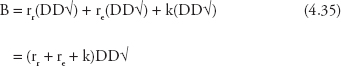
Solving 4.35 for DD√ yields 4.36. This expression for DD√ is substituted into 4.37, an equation for the M1 measure of money. The result is 4.38, the basic money supply model for M1-money. The term in brackets is the money supply multiplier (m).

Given recent changes impacting on reserve ratio requirements in this country, an alternative version of the money multiplier is also included. It is the multiplier in 4.22 above. This multiplier uses an aggregate reserve ratio (r) for banks. That is, let r = r_r + r_e. Substitution of r into 4.38 yields this second money multiplier.