
Now that we are familiar with epipolar geometry, let's see how to use it to build a 3D map based on stereo images. Let's consider the following figure:

The first step is to extract the disparity map between the two images. If you look at the figure, as we go closer to the object from the cameras along the connecting lines, the distance decreases between the points. Using this information, we can infer the distance of each point from the camera. This is called a depth map. Once we find the matching points between the two images, we can find the disparity by using epipolar lines to impose epipolar constraints.
Let's consider the following image:

If we capture the same scene from a different position, we get the following image:

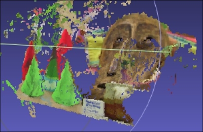
If we reconstruct the 3D map, it will look like this:

Bear in mind that these images were not captured using perfectly aligned stereo cameras. That's the reason the 3D map looks so noisy! This is just to demonstrate how we can reconstruct the real world using stereo images. Let's consider an image pair captured using stereo cameras that are properly aligned. Following is the left view image:

Next is the corresponding right view image:

If you extract the depth information and build the 3D map, it will look like this:

Let's rotate it to see if the depth is right for the different objects in the scene:
You need a software called MeshLab to visualize the 3D scene. We'll discuss about it soon. As we can see in the preceding images, the items are correctly aligned according to their distance from the camera. We can intuitively see that they are arranged in the right way, including the tilted position of the mask. We can use this technique to build many interesting things.
Let's see how to do it in OpenCV-Python:
import argparse

import cv2
import numpy as np

def build_arg_parser():
    parser = argparse.ArgumentParser(description='Reconstruct the 3D map from
            the two input stereo images. Output will be saved in 'output.ply'')
    parser.add_argument("--image-left", dest="image_left", required=True,
            help="Input image captured from the left")
    parser.add_argument("--image-right", dest="image_right", required=True,
            help="Input image captured from the right")
    parser.add_argument("--output-file", dest="output_file", required=True,
            help="Output filename (without the extension) where the point cloud will be saved")
    return parser

def create_output(vertices, colors, filename):
    colors = colors.reshape(-1, 3)
    vertices = np.hstack([vertices.reshape(-1,3), colors])

    ply_header = '''ply
        format ascii 1.0
        element vertex %(vert_num)d
        property float x
        property float y
        property float z
        property uchar red
        property uchar green
        property uchar blue
        end_header
    '''

    with open(filename, 'w') as f:
        f.write(ply_header % dict(vert_num=len(vertices)))
        np.savetxt(f, vertices, '%f %f %f %d %d %d')

if __name__ == '__main__':
    args = build_arg_parser().parse_args()
    image_left = cv2.imread(args.image_left)
    image_right = cv2.imread(args.image_right)
    output_file = args.output_file + '.ply'

    if image_left.shape[0] != image_right.shape[0] or
            image_left.shape[1] != image_right.shape[1]:
        raise TypeError("Input images must be of the same size")

    # downscale images for faster processing
    image_left = cv2.pyrDown(image_left)
    image_right = cv2.pyrDown(image_right)

    # disparity range is tuned for 'aloe' image pair
    win_size = 1
    min_disp = 16
    max_disp = min_disp * 9
    num_disp = max_disp - min_disp   # Needs to be divisible by 16
    stereo = cv2.StereoSGBM(minDisparity = min_disp,
        numDisparities = num_disp,
        SADWindowSize = win_size,
        uniquenessRatio = 10,
        speckleWindowSize = 100,
        speckleRange = 32,
        disp12MaxDiff = 1,
        P1 = 8*3*win_size**2,
        P2 = 32*3*win_size**2,
        fullDP = True
    )

    print "
Computing the disparity map ..."
    disparity_map = stereo.compute(image_left, image_right).astype(np.float32) / 16.0

    print "
Generating the 3D map ..."
    h, w = image_left.shape[:2]
    focal_length = 0.8*w

    # Perspective transformation matrix
    Q = np.float32([[1, 0, 0, -w/2.0],
                    [0,-1, 0,  h/2.0],
                    [0, 0, 0, -focal_length],
                    [0, 0, 1, 0]])

    points_3D = cv2.reprojectImageTo3D(disparity_map, Q)
    colors = cv2.cvtColor(image_left, cv2.COLOR_BGR2RGB)
    mask_map = disparity_map > disparity_map.min()
    output_points = points_3D[mask_map]
    output_colors = colors[mask_map]

    print "
Creating the output file ...
"
    create_output(output_points, output_colors, output_file)
To visualize the output, you need to download MeshLab from http://meshlab.sourceforge.net.
Just open the output.ply file using MeshLab and you'll see the 3D image. You can rotate it to get a complete 3D view of the reconstructed scene. Some of the alternatives to MeshLab are Sketchup on OS X and Windows, and Blender on Linux.