
C H A P T E R 9
Manually Tuning SQL
It has been said many times in books, articles, and other publications that over 90% of all performance problems on a database are due to poorly written SQL. Often, database administrators are given the task of “fixing the database” when queries are not performing adequately. The database administrator is often guilty before proven innocent—and often has the task of proving that a performance problem is not the database itself, but rather, simply, SQL statements that are not written efficiently. The goal, of course, is to have SQL statements written efficiently the first time. This chapter's focus is to help monitor and analyze existing queries to help show why they may be underperforming, as well as show some steps to improve queries.
If you have SQL code that you are maintaining or that needs help to improve performance, some of the questions that need to be asked first include the following:
- Has the query run before successfully?
- Was the query performance acceptable in the past?
- Are there any metrics on how long the query has run when successful?
- How much data is typically returned from the query?
- When was the last time statistics were gathered on the objects referenced in the query?
Once these questions are answered, it helps to direct the focus to where the problem may lie. You then may want to run an explain plan for the query to see if the execution plan is reasonable at first glance. The skill of reading an explain plan takes time and improves with experience. Sometimes, especially if there are views on top of the objects being queried, an explain plan can be lengthy and intimidating. Therefore, it's important to simply know what to look for first, and then dig as you go.
At times, poorly running SQL can expose database configuration issues, but normally, poorly performing SQL queries occur due to poorly written SQL statements. Again, as a database administrator or database developer, the best approach is to take time up front whenever possible to tune the SQL statements prior to ever running in a production environment. Often, a query's elapsed time is a benchmark for efficiency, which is an easy trap in which to fall. Over time, database characteristics change, more historical data may be stored for an application, and a query that performed well on initial install simply doesn't scale as an application matures. Therefore, it's important to take the time to do it right the first time, which is easy to say, but tough to accomplish when balancing client requirements, budgets, and project timelines.
9-1. Displaying an Execution Plan for a Query
Problem
You want to quickly retrieve an execution plan from within SQL Plus for a query.
Solution
From within SQL Plus, you can use the AUTOTRACE feature to quickly retrieve the execution plan for a query. This SQL Plus utility is very handy at getting the execution plan, along with getting statistics for the query's execution plan. In the most basic form, to enable AUTOTRACE within your session, execute the following command within SQL Plus:
SQL> set autotrace on
Then, you can run a query using AUTOTRACE, which will show the execution plan and query execution statistics for your query:
SELECT last_name, first_name

FROM employees NATURAL JOIN departments

WHERE employee_id = 101;


LAST_NAME                 FIRST_NAME

------------------------- --------------------

Kochhar                   Neena


--------------------------------------------------------------------------------------------

| Id  | Operation                    | Name          | Rows  | Bytes | Cost (%CPU)| Time   |

--------------------------------------------------------------------------------------------

|   0 | SELECT STATEMENT             |               |     1 |    33 |     2   (0)| 00:00:01

|   1 |  NESTED LOOPS                |               |     1 |    33 |     2   (0)| 00:00:01

|   2 |   TABLE ACCESS BY INDEX ROWID| EMPLOYEES     |     1 |    26 |     1   (0)| 00:00:01

|*  3 |    INDEX UNIQUE SCAN         | EMP_EMP_ID_PK |     1 |       |     0   (0)| 00:00:01

|*  4 |   TABLE ACCESS BY INDEX ROWID| DEPARTMENTS   |    11 |    77 |     1   (0)| 00:00:01

|*  5 |    INDEX UNIQUE SCAN         | DEPT_ID_PK    |     1 |       |     0   (0)| 00:00:01

--------------------------------------------------------------------------------------------


Statistics

----------------------------------------------------------

          0  recursive calls

          0  db block gets

          4  consistent gets

          0  physical reads

          0  redo size

        490  bytes sent via SQL*Net to client

        416  bytes received via SQL*Net from client

          2  SQL*Net roundtrips to/from client

          0  sorts (memory)

          0  sorts (disk)

          1  rows processed
How It Works
There are several options to choose from when using AUTOTRACE, and the basic factors are as follows:
- Do you want to execute the query?
- Do you want to see the execution plan for the query?
- Do you want to see the execution statistics for the query?
As you can see from Table 9-1, you can abbreviate each command, if so desired. The portions of the words in brackets are optional.

The most common use for AUTOTRACE is to get the execution plan for the query, without running the query. By doing this, you can quickly see whether you have a reasonable execution plan, and can do this without having to execute the query:
SQL> set autot trace exp


SELECT l.location_id, city, department_id, department_name

  FROM locations l, departments d

  WHERE l.location_id = d.location_id(+)

  ORDER BY 1;
-----------------------------------------------------------------------------------

| Id  | Operation           | Name        | Rows  | Bytes | Cost (%CPU)| Time     |

-----------------------------------------------------------------------------------

|   0 | SELECT STATEMENT    |             |    27 |   837 |     8  (25)| 00:00:01 |

|   1 |  SORT ORDER BY      |             |    27 |   837 |     8  (25)| 00:00:01 |

|*  2 |   HASH JOIN OUTER   |             |    27 |   837 |     7  (15)| 00:00:01 |

|   3 |    TABLE ACCESS FULL| LOCATIONS   |    23 |   276 |     3   (0)| 00:00:01 |

|   4 |    TABLE ACCESS FULL| DEPARTMENTS |    27 |   513 |     3   (0)| 00:00:01 |

-----------------------------------------------------------------------------------
For the foregoing query, if you wanted to see only the execution statistics for the query, and did not want to see all the query output, you would do the following:
SQL> set autot trace stat

SQL> /


43 rows selected.


Statistics

----------------------------------------------------------

          0  recursive calls

          0  db block gets

         14  consistent gets

          0  physical reads

          0  redo size

       1862  bytes sent via SQL*Net to client

        438  bytes received via SQL*Net from client

          4  SQL*Net roundtrips to/from client

          1  sorts (memory)

          0  sorts (disk)

         43  rows processed
Once you are done using AUTOTRACE for a given session and want to turn it off and run other queries without using AUTOTRACE, run the following command from within your SQL Plus session:
SQL> set autot off
The default for each SQL Plus session is AUTOTRACE OFF, but if you want to check to see what your current AUTOTRACE setting is for a given session, you can do that by executing the following command:
SQL> show autot

autotrace OFF
9-2. Customizing Execution Plan Output
Problem
You want to configure the explain plan output for your query based on your specific needs.
Solution
The Oracle-provided PL/SQL package DBMS_XPLAN has extensive functionality to get explain plan information for a given query. There are many functions within the DBMS_XPLAN package. The DISPLAY function can be used to quickly get the execution plan for a query, and also to customize the information that is presented to meet your specific needs. The following is an example that invokes the basic display functionality:
explain plan for

SELECT last_name, first_name

FROM employees JOIN departments USING(department_id)

WHERE employee_id = 101;


Explained.


SELECT * FROM table(dbms_xplan.display);


PLAN_TABLE_OUTPUT

--------------------------------------------------------------------------------------------

Plan hash value: 1833546154


--------------------------------------------------------------------------------------------

| Id  | Operation                   | Name          | Rows  | Bytes | Cost (%CPU)| Time    |

--------------------------------------------------------------------------------------------

|   0 | SELECT STATEMENT            |               |     1 |    22 |     1   (0)| 00:00:01|

|*  1 |  TABLE ACCESS BY INDEX ROWID| EMPLOYEES     |     1 |    22 |     1   (0)| 00:00:01|

|*  2 |   INDEX UNIQUE SCAN         | EMP_EMP_ID_PK |     1 |       |     0   (0)| 00:00:01|

--------------------------------------------------------------------------------------------


Predicate Information (identified by operation id):

---------------------------------------------------


   1 - filter("EMPLOYEES"."DEPARTMENT_ID" IS NOT NULL)

   2 - access("EMPLOYEES"."EMPLOYEE_ID"=101)
The DBMS_XPLAN.DISPLAY procedure is very flexible in configuring how you would like to see output. If you wanted to see only the most basic execution plan output, using the foregoing query, you could configure the DBMS_XPLAN.DISPLAY function to get that output:
SELECT * FROM table(dbms_xplan.display(null,null,'BASIC'));


-----------------------------------------------------

| Id  | Operation                   | Name          |

-----------------------------------------------------

|   0 | SELECT STATEMENT            |               |

|   1 |  TABLE ACCESS BY INDEX ROWID| EMPLOYEES     |

|   2 |   INDEX UNIQUE SCAN         | EMP_EMP_ID_PK |

-----------------------------------------------------
How It Works
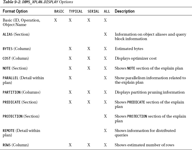
The DBMS_XPLAN.DISPLAY function has a lot of built-in functionality to provide customized output based on your needs. The function provides four basic levels of output detail:
BASIC- TYPICAL (default)
SERIAL- ALL
Table 9-2 shows the format options that are included within each level of detail option.
If you simply want the default output format, there is no need to pass in any special format options:
SELECT * FROM table(dbms_xplan.display);
If you want to get all available output for a query, use the ALL level of detail format output option:
SELECT * FROM table(dbms_xplan.display(null,null,'ALL'));


--------------------------------------------------------------------------------------------

| Id  | Operation                   | Name          | Rows  | Bytes | Cost (%CPU)| Time    |

--------------------------------------------------------------------------------------------

|   0 | SELECT STATEMENT            |               |     1 |    22 |     1   (0)| 00:00:01|

|*  1 |  TABLE ACCESS BY INDEX ROWID| EMPLOYEES     |     1 |    22 |     1   (0)| 00:00:01|

|*  2 |   INDEX UNIQUE SCAN         | EMP_EMP_ID_PK |     1 |       |     0   (0)| 00:00:01|

--------------------------------------------------------------------------------------------


Query Block Name / Object Alias (identified by operation id):

-------------------------------------------------------------


   1 - SEL$38D4D5F3 / EMPLOYEES@SEL$1

   2 - SEL$38D4D5F3 / EMPLOYEES@SEL$1


Predicate Information (identified by operation id):

---------------------------------------------------


   1 - filter("EMPLOYEES"."DEPARTMENT_ID" IS NOT NULL)

   2 - access("EMPLOYEES"."EMPLOYEE_ID"=101)


Column Projection Information (identified by operation id):

-----------------------------------------------------------


   1 - "EMPLOYEES"."FIRST_NAME"[VARCHAR2,20], "EMPLOYEES"."LAST_NAME"[VARCHAR2,25]

   2 - "EMPLOYEES".ROWID[ROWID,10]


Note

-----

   - rule based optimizer used (consider using cbo)
One of the very nice features of the DBMS_XPLAN.DISPLAY function is after deciding the base level of detail you need, you can add individual options to be displayed in addition to the base output for that level of detail. For instance, if you want just the most basic output information, but also want to know cost information, you can format the DBMS_XPLAN.DISPLAY as follows:
SELECT * FROM table(dbms_xplan.display(null,null,'BASIC +COST'));
--------------------------------------------------------------------------------

| Id  | Operation                    | Name                       | Cost (%CPU)|

--------------------------------------------------------------------------------

|   0 | SELECT STATEMENT             |                            |     1   (0)|

|   1 |  RESULT CACHE                | 0fnzzb94z0dj2b5vzkmq4f4xcu |            |

|   2 |   TABLE ACCESS BY INDEX ROWID| EMPLOYEES                  |     1   (0)|

|   3 |    INDEX UNIQUE SCAN         | EMP_EMP_ID_PK              |     0   (0)|

--------------------------------------------------------------------------------
You can also do the reverse, that is, subtract information you do not want to see. If you wanted to see the output using the TYPICAL level of output, but did not want to see the ROWS or BYTES information, you could issue the following query to display that level of output:
SELECT * FROM table(dbms_xplan.display(null,null,'TYPICAL -BYTES -ROWS'));


-----------------------------------------------------------------------------

| Id  | Operation                   | Name          | Cost (%CPU)| Time     |

-----------------------------------------------------------------------------

|   0 | SELECT STATEMENT            |               |     1   (0)| 00:00:01 |

|*  1 |  TABLE ACCESS BY INDEX ROWID| EMPLOYEES     |     1   (0)| 00:00:01 |

|*  2 |   INDEX UNIQUE SCAN         | EMP_EMP_ID_PK |     0   (0)| 00:00:01 |

-----------------------------------------------------------------------------
9-3. Graphically Displaying an Execution Plan
Problem
You want to quickly view an execution plan without having to run SQL statements to retrieve the execution plan. You would like to use a GUI to view the plan, so that you can just click your way to it.
Solution
From within Enterprise Manager, you can quickly find the execution plan for a query. In order to use this functionality, you will have to have Enterprise Manager configured within your environment. This can be either Database Control, which manages a single database, or Grid Control, which manages an enterprise of databases. In order to see the execution plan for a given query, you will need to navigate to the Top Sessions screen of Enterprise Manager. (Refer to the Oracle Enterprise Manager documentation for your specific release.) Once on the Top Sessions screen, you can drill down into session specific information. First, find your session. Then, click the SQL ID shown under Current SQL. From there, you can click Plan, and the execution plan will appear, such as the one shown in Figure 9-1.

Figure 9-1. Sample execution plan output from within Enterprise Manager
How It Works
Using Enterprise Manager makes it very easy to find the execution plan for currently running SQL operations within your database. If a particular SQL statement isn't performing as expected, this method is one of the fastest ways to determine the execution plan for a running query or other SQL operation. In order to use this feature, you must be licensed for the Tuning Pack of Enterprise Manager.
9-4. Reading an Execution Plan
Problem
You have run an explain plan for a given SQL statement, and want to understand how to read the plan.
Solution
The execution plan for a SQL operation tells you step-by-step exactly how the Oracle optimizer will execute your SQL operation. Using AUTOTRACE, let's get an explain plan for the following query:
set autotrace trace explain


SELECT ename, dname

FROM emp JOIN dept USING (deptno);


----------------------------------------------------------------------------------------

| Id  | Operation                    | Name    | Rows  | Bytes | Cost (%CPU)| Time     |

----------------------------------------------------------------------------------------

|   0 | SELECT STATEMENT             |         |    14 |   308 |     6  (17)| 00:00:01 |

|   1 |  MERGE JOIN                  |         |    14 |   308 |     6  (17)| 00:00:01 |

|   2 |   TABLE ACCESS BY INDEX ROWID| DEPT    |     4 |    52 |     2   (0)| 00:00:01 |

|   3 |    INDEX FULL SCAN           | PK_DEPT |     4 |       |     1   (0)| 00:00:01 |

|*  4 |   SORT JOIN                  |         |    14 |   126 |     4  (25)| 00:00:01 |

|   5 |    TABLE ACCESS FULL         | EMP     |    14 |   126 |     3   (0)| 00:00:01 |

----------------------------------------------------------------------------------------


Predicate Information (identified by operation id):

---------------------------------------------------


   4 - access("EMP"."DEPTNO"="DEPT"."DEPTNO")

       filter("EMP"."DEPTNO"="DEPT"."DEPTNO")


Note

-----

   - automatic DOP: Computed Degree of Parallelism is 1 because of parallel threshold
Once you have an explain plan to interpret, you can tell which steps are executed first because the innermost or most indented steps are executed first, and are executed from the inside out, in top-down order. In the foregoing query, we are joining the EMP and DEPT tables. Here are the steps of how the query is processed based on the execution plan:
- The
PK_DEPTindex is scanned (ID 3). - All
EMPtable rows are scanned (ID 5). - Rows are retrieved from the
DEPTtable based on the matching entries in thePK_DEPTindex (ID 2). - Resulting data from the
EMPtable is sorted (ID 4). - Data from the
EMPandDEPTtables are then joined via aMERGE JOIN(ID 1). - The resulting data from the query is returned to the user (ID 0).
How It Works
When first looking at an explain plan and wanting to quickly get an idea of the steps in which the query will be executed, do the following:
- Look for the most indented rows in the plan (the right-most rows). These will be executed first.
- If multiple rows are at the same level of indentation, they will be executed in top-down fashion in the plan, with the highest rows in the plan first moving downward in the plan.
- Look at the next most indented row or rows and continue working your way outward.
- The top of the explain plan corresponds with the least indented or left-most part of the plan, and usually is where the results are returned to the user.
Once you have an explain plan for a query, and can understand the sequence of how the query will be processed, you then can move on and perform some analysis to determine if the explain plan you are looking at is efficient. When looking at your explain plan, answer these questions and consider these factors when determining if you have an efficient plan:
- What is the access path for the query (is the query performing a full table scan or is the query using an index)?
- What is the join method for the query (if a join condition is present)?
- Look at the columns within the filtering criteria found within the
WHEREclause of the query, and determine if they are indexed. - Get the volume or number of rows for each table in the query. Are the tables small, medium-sized, or large? This may help you determine the most appropriate join method. See Table 9-3 for a synopsis of the types of join methods.
- When were statistics last gathered for the objects involved in the query?
- Look at the
COSTcolumn of the explain plan to get a starting cost.
By looking at our original explain plan, we determined that the EMP table is larger in size, and also that there is no index present on the DEPTNO column, which is used within a join condition between the DEPT and EMP tables. By placing an index on the DEPTNO column on the EMP table and gathering statistics on the EMP table, the plan now uses an index:
---------------------------------------------------------------------------------------

| Id  | Operation                    | Name   | Rows  | Bytes | Cost (%CPU)| Time     |

---------------------------------------------------------------------------------------

|   0 | SELECT STATEMENT             |        |    14 |   280 |     6  (17)| 00:00:01 |

|   1 |  MERGE JOIN                  |        |    14 |   280 |     6  (17)| 00:00:01 |

|   2 |   TABLE ACCESS BY INDEX ROWID| EMP    |    14 |    98 |     2   (0)| 00:00:01 |

|   3 |    INDEX FULL SCAN           | EMP_I2 |    14 |       |     1   (0)| 00:00:01 |

|*  4 |   SORT JOIN                  |        |     4 |    52 |     4  (25)| 00:00:01 |

|   5 |    TABLE ACCESS FULL         | DEPT   |     4 |    52 |     3   (0)| 00:00:01 |

---------------------------------------------------------------------------------------

For information on parallel execution plans, see Chapter 15.
![]() Tip One of the most common reasons for a sub-optimal explain plan is the lack of current statistics on one or more objects involved in a query.
Tip One of the most common reasons for a sub-optimal explain plan is the lack of current statistics on one or more objects involved in a query.
9-5. Monitoring Long-Running SQL Statements
Problem
You have a SQL statement that runs a long time, and you want to be able to monitor the progress of the statement and find out when it will finish.
Solution
By viewing information for a long-running query in the V$SESSION_LONGOPS data dictionary view, you can gauge about when a query will finish. Let's say you are running the following query, with join conditions, against a large table:
SELECT last_name, first_name FROM employees_big

WHERE last_name = 'EVANS';
With a simple query against the V$SESSION_LONGOPS view, you can quickly get an idea of how long the query will execute, and when it will finish:
SELECT username, target, sofar blocks_read, totalwork total_blocks,

round(time_remaining/60) minutes

FROM v$session_longops

WHERE sofar <> totalwork

and username = 'HR';


USERNAME     TARGET               BLOCKS_READ TOTAL_BLOCKS    MINUTES

------------ -------------------- ----------- ------------ ----------

HR           HR.EMPLOYEES_BIG           81101      2353488         10
As the query progresses, you can see the BLOCKS_READ column increase, as well as the MINUTES column decrease. It is usually necessary to place the WHERE clause to eliminate rows that have been completed, which is why in the foregoing query it asked for rows where the SOFAR column did not equal TOTALWORK.
How It Works
In order to be able to monitor a query within the V$SESSION_LONGOPS view, the following requirements apply:
- The query must run for six seconds or greater.
- The table being accessed must be greater than 10,000 database blocks.
TIMED_STATISTICSmust be set orSQL_TRACEmust be turned on.- The objects within the query must have been analyzed via
DBMS_STATSorANALYZE.
This view can contain information on SELECT statements, DML statements such as UPDATE, as well as DDL statements such as CREATE INDEX. Some common operations that find themselves in the V$SESSION_LONGOPS view include table scans, index scans, join operations, parallel operations, RMAN backup operations, sort operations, and Data Pump operations.
9-6. Identifying Resource-Consuming SQL Statements That Are Currently Executing
Problem
You have contention issues within your database, and want to identify the SQL statement consuming the most system resources.
![]() Note Recipe 9-9 shows how to examine the historical record to find resource-consuming SQL statements that have executed in the past, but that are not currently executing.
Note Recipe 9-9 shows how to examine the historical record to find resource-consuming SQL statements that have executed in the past, but that are not currently executing.
Solution
Look at the V$SQLSTATS view, which gives information about currently or recently run SQL statements. If you wanted to get the top five recent SQL statements that performed the highest disk I/O, you could issue the following query:
SELECT sql_text, disk_reads FROM

  (SELECT sql_text, buffer_gets, disk_reads, sorts,

   cpu_time/1000000 cpu, rows_processed, elapsed_time

   FROM v$sqlstats

   ORDER BY disk_reads DESC)

WHERE rownum <= 5;
If you wanted to see the top five SQL statements by CPU time, sorts, loads, invalidations, or any other column, simply replace the disk_reads column in the foregoing query with your desired column. The SQL_TEXT column can make the results look messy, so another alternative is to substitute the SQL_TEXT column with SQL_ID, and then, based on the statistics shown, you can run a query to simply get the SQL_TEXT based on a given SQL_ID.
How It Works
The V$SQLSTATS view is meant to help more quickly find information on resource-consuming SQL statements. V$SQLSTATS has the same information as the V$SQL and V$SQLAREA views, but V$SQLSTATS has only a subset of columns of the other views. However, data is held within the V$SQLSTATS longer than either V$SQL or V$SQLAREA.
Sometimes, there are SQL statements that are related to the database background processing of keeping the database running, and you may not want to see those statements, but only the ones related to your application. If you join V$SQLSTATS to V$SQL, you can see information for particular users. See the following example:
SELECT schema, sql_text, disk_reads, round(cpu,2) FROM

  (SELECT s.parsing_schema_name schema, t.sql_id, t.sql_text, t.disk_reads,

  t.sorts, t.cpu_time/1000000 cpu, t.rows_processed, t.elapsed_time

   FROM v$sqlstats t join v$sql s on(t.sql_id = s.sql_id)

  WHERE parsing_schema_name = 'SCOTT'

  ORDER BY disk_reads DESC)

WHERE rownum <= 5;
Keep in mind that V$SQL represents SQL held in the shared pool, and is aged out faster than the data in V$SQLSTATS, so this query will not return data for SQL that has been already aged out of the shared pool.
9-7. Seeing Execution Statistics for Currently Running SQL
Problem
You want to view execution statistics for SQL statements that are currently running.
Solution
You can use the V$SQL_MONITOR view to see real-time statistics of currently running SQL, and see the resource consumption used for a given query based on such statistics as CPU usage, buffer gets, disk reads, and elapsed time of the query. Let's first find a current executing query within our database:
SELECT sid, sql_text FROM v$sql_monitor

WHERE status = 'EXECUTING';


       SID SQL_TEXT

---------- -----------------------------------------------------------------

       100 select department_name, city, avg(salary)

           from employees_big join departments using(department_id)

           join locations using (location_id)

           group by department_name, city

           having avg(salary) > 2000

           order by 2,1
For the foregoing executing query found in V$SQL_MONITOR, we can see the resource utilization for that statement as it executes:
SELECT sid, buffer_gets, disk_reads, round(cpu_time/1000000,1) cpu_seconds

FROM v$sql_monitor

WHERE SID=100

AND status = 'EXECUTING';


       SID BUFFER_GETS DISK_READS CPU_SECONDS

---------- ----------- ---------- -----------

       100      149372       4732        39.1
The V$SQL_MONITOR view contains currently running SQL statements, as well as recently run SQL statements. If you wanted to see the top five most CPU-consuming queries in your database, you could issue the following query:
SELECT * FROM (

  SELECT sid, buffer_gets, disk_reads, round(cpu_time/1000000,1) cpu_seconds

  FROM v$sql_monitor

  ORDER BY cpu_time desc)

WHERE rownum <= 5;


       SID BUFFER_GETS DISK_READS CPU_SECONDS

---------- ----------- ---------- -----------

        20     1332665      30580       350.5

       105      795330      13651       269.7

        20      259324       5449        71.6

        20      259330       5485        71.3

       100      259236       8188        67.9
How It Works
SQL statements are monitored in V$SQL_MONITOR under the following conditions:
- Automatically for any parallelized statements
- Automatically for any DML or DDL statements
- Automatically if a particular SQL statement has consumed at least five seconds of CPU or I/O time
- Monitored for any SQL statement that has monitoring set at the statement level
To turn monitoring on at the statement level, a hint can be used. See the following example:
SELECT /*+ monitor */ ename, dname

FROM emppart JOIN dept USING (deptno);
If, for some reason, you do not want certain statements monitored, you can use the NOMONITOR hint in the statement to prevent monitoring from occurring for a given statement.
Statistics in V$SQL_MONITOR are updated near real-time, that is, every second. Any currently executing SQL statement that is being monitored can be found in V$SQL_MONITOR. Completed queries can be found there for at least one minute after execution ends, and can exist there longer, depending on the space requirements needed for newly executed queries. One key advantage of the V$SQL_MONITOR view is it has detailed statistics for each and every execution of a given query, unlike V$SQL, where results are cumulative for several executions of a SQL statement. In order to drill down, then, to a given execution of a SQL statement, you need three columns from V$SQL_MONITOR:
SQL_IDSQL_EXEC_STARTSQL_EXEC_ID
If we wanted to see all executions for a given query (based on the SQL_ID column), we can get that information by querying on the three necessary columns to drill to a given execution of a SQL query:
SELECT * FROM (

  SELECT sql_id, to_char(sql_exec_start,'yyyy-mm-dd:hh24:mi:ss') sql_exec_start,

         sql_exec_id, sum(buffer_gets) buffer_gets,

         sum(disk_reads) disk_reads, round(sum(cpu_time/1000000),1) cpu_secs

  FROM v$sql_monitor

  WHERE sql_id = 'fcg00hyh7qbpz'

  GROUP BY sql_id, sql_exec_start, sql_exec_id

  ORDER BY 6 desc)

WHERE rownum <= 5;


SQL_ID        SQL_EXEC_START      SQL_EXEC_ID BUFFER_GETS DISK_READS CPU_SECS

------------- ------------------- ----------- ----------- ---------- --------

fcg00hyh7qbpz 2011-05-21:12:28:10    16777222      259324       5449     71.6

fcg00hyh7qbpz 2011-05-21:12:29:24    16777223      259330       5485     71.3

fcg00hyh7qbpz 2011-05-21:12:26:08    16777220      213823       4502     58.4

fcg00hyh7qbpz 2011-05-21:12:27:09    16777221      211752       4579     58.1

fcg00hyh7qbpz 2011-05-21:12:25:37    16777219      107973       2414     29.4
Keep in mind that if a statement is running in parallel, one row will appear for each parallel thread for the query, including one for the query coordinator. However, they will share the same SQL_ID, SQL_EXEC_START, and SQL_EXEC_ID values. In this case, you could perform an aggregation on a particular statistic, if desired. See the following example for a parallelized query, along with parallel slave information denoted by the PX_SERVER# column:
SELECT sql_id, sql_exec_start, sql_exec_id, px_server# px#, disk_reads,

       cpu_time/1000000 cpu_secs, buffer_gets

FROM v$sql_monitor

WHERE status = 'EXECUTING'

ORDER BY px_server#;


SQL_ID        SQL_EXEC_S SQL_EXEC_ID PX# DISK_READS CPU_SECS BUFFER_GETS

------------- ---------- ----------- --- ---------- -------- -----------

0gzf8010xdasr 2011-05-21    16777216   1       4306     38.0      136303

0gzf8010xdasr 2011-05-21    16777216   2       4625     40.6      146497

0gzf8010xdasr 2011-05-21    16777216   3       4774     41.6      149717

0gzf8010xdasr 2011-05-21    16777216   4       4200     37.6      132167

0gzf8010xdasr 2011-05-21    16777216              6     92.2          53
Then, to perform a simple aggregation for a given query, in this case, our parallelized query, the aggregation is done on the three key columns that make up a single execution of a given SQL statement:
SELECT sql_id,sql_exec_start, sql_exec_id, sum(buffer_gets) buffer_gets,

       sum(disk_reads) disk_reads, round(sum(cpu_time/1000000),1) cpu_seconds

FROM v$sql_monitor

WHERE sql_id = '0gzf8010xdasr'

GROUP BY sql_id, sql_exec_start, sql_exec_id;


SQL_ID        SQL_EXEC_S SQL_EXEC_ID BUFFER_GETS DISK_READS CPU_SECONDS

------------- ---------- ----------- ----------- ---------- -----------

0gzf8010xdasr 2011-05-21    16777216      642403      20351       283.7
If you wanted to perform an aggregation for one SQL statement, regardless of the number of times is has been executed, simply run the aggregate query only on the SQL_ID column, as shown here:
SELECT sql_id, sum(buffer_gets) buffer_gets,

       sum(disk_reads) disk_reads, round(sum(cpu_time/1000000),1) cpu_seconds

FROM v$sql_monitor

WHERE sql_id = '0gzf8010xdasr'

GROUP BY sql_id;
![]() Note Initialization parameter
Note Initialization parameter STATISTICS_LEVEL must be set to TYPICAL or ALL, and CONTROL_MANAGEMENT_PACK_ACCESS must be set to DIAGNOSTIC+TUNING for SQL monitoring to occur.
9-8. Monitoring Progress of a SQL Execution Plan
Problem
You want to see the progress a query is making from within the execution plan used.
Solution
There are a couple of ways to get information to see where a query is executing in terms of the execution plan. First, by querying the V$SQL_PLAN_MONITOR view, you can get information for all queries that are in progress, as well as recent queries that are complete. If we are joining two tables to get employee and department information, our query would look like this:
SELECT ename, dname

FROM emppart JOIN dept USING (deptno);


--------------------------------------------

| Id  | Operation               | Name     |

--------------------------------------------

|   0 | SELECT STATEMENT        |          |

|   1 |  PX COORDINATOR         |          |

|   2 |   PX SEND QC (RANDOM)   | :TQ10001 |

|   3 |    HASH JOIN            |          |

|   4 |     BUFFER SORT         |          |

|   5 |      PX RECEIVE         |          |

|   6 |       PX SEND BROADCAST | :TQ10000 |

|   7 |        TABLE ACCESS FULL| DEPT     |

|   8 |     PX BLOCK ITERATOR   |          |

|   9 |      TABLE ACCESS FULL  | EMPPART  |

--------------------------------------------
To see information for the foregoing query while it is currently running, you can issue a query like the one shown here (some rows have been removed for conciseness):
column operation format a25

column plan_line_id format 9999 heading 'LINE'

column plan_options format a10 heading 'OPTIONS'

column status format a10

column output_rows heading 'ROWS'

break on sid on sql_id on status


SELECT sid, sql_id, status, plan_line_id,

plan_operation || ' ' || plan_options operation, output_rows

FROM v$sql_plan_monitor

WHERE status not like '%DONE%'

ORDER BY 1,4;
       SID SQL_ID        STATUS      LINE OPERATION                       ROWS

---------- ------------- ---------- ----- ------------------------- ----------

        18 36bdwxutr5n75 EXECUTING      0 SELECT STATEMENT             3929326

                                        1 PX COORDINATOR               3929326

        27 36bdwxutr5n75 EXECUTING      0 SELECT STATEMENT                   0

                                        2 PX SEND QC (RANDOM)          1752552

                                        3 HASH JOIN                    1752552

                                        8 PX BLOCK ITERATOR            1752552

                                        9 TABLE ACCESS FULL            1752552

       101 36bdwxutr5n75 EXECUTING      0 SELECT STATEMENT                   0

                                        2 PX SEND QC (RANDOM)          2148232

                                        3 HASH JOIN                    2148232

                                        8 PX BLOCK ITERATOR            2148232

                                        9 TABLE ACCESS FULL            2148232
In this particular example, the EMPPART table has a parallel degree of 2, and we can see that for SIDs 27 and 101, these are the parallel slaves that are getting the data. As these processes pass data back to the query coordinator and then back to the user, we can see that when we look at SID 18. If we simply run subsequent queries against the V$SQL_PLAN_MONITOR view, we can see the progress of the query as it is executing. In the foregoing example, we simply see the output row values increasing as the query progresses.
Another method of seeing the progress of a query via the execution plan is by using the DBMS_SQLTUNE.REPORT_SQL_MONITOR function. If we use the same query against the EMPPART and DEPT tables used in the previous example, we can run the REPORT_SQL_MONITOR function to get a graphical look at the progress. See the following example of how to generate the file that would produce the HTML file that could be, in turn, used to view our progress. Figure 9-2 shows portions of the resulting report.
set pages 9999

set long 1000000

SELECT DBMS_SQLTUNE.REPORT_SQL_MONITOR(sql_id=> '36bdwxutr5n75',type=>'HTML') FROM dual;
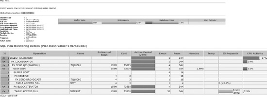
Figure 9-2. Sample HTML report from DBMS_SQLTUNE.REPORT_SQL_MONITOR
How It Works
The V$SQL_PLAN_MONITOR is populated from the V$SQL_MONITOR view (see Recipe 9-7). Both of these views are new as of Oracle 11g, and are updated every second that a statement executes. The V$SQL_MONITOR view is populated each time a SQL statement is monitored.
The DBMS_SQLTUNE.REPORT_SQL_MONITOR function can be invoked in several ways. The level of detail, as well as the type of detail you wish to see in the report, can be changed based on the parameters passed into the function. The output can be viewed in several formats, including plain text, HTML, and XML. The default output format is plain text. As an example, let's say we wanted to see the output for our join against the EMPPART and DEPT tables. In this instance, we want the output in text format. We want the detail aggregated, and we want to see just the most basic level of detail. Our query would then be run as follows:
SELECT DBMS_SQLTUNE.REPORT_SQL_MONITOR

(sql_id=>'36bdwxutr5n75',event_detail=>'NO',report_level=>'BASIC') FROM dual;


SQL Monitoring Report


SQL Text

------------------------------

select ename, dname from emppart join dept using (deptno)


Global Information

------------------------------

 Status              :  EXECUTING

 Instance ID         :  1

 Session             :  SCOTT (27:229)

 SQL ID              :  36bdwxutr5n75

 SQL Execution ID    :  16777225

 Execution Started   :  05/15/2011 14:56:16

 First Refresh Time  :  05/15/2011 14:56:16

 Last Refresh Time   :  05/15/2011 15:09:47

 Duration            :  812s

 Module/Action       :  SQL*Plus/-

 Service             :  SYS$USERS

 Program             :  sqlplus@ora

 Fetch Calls         :  6131367


Global Stats

==========================================================================================

| Elapsed |   Cpu   |    IO    | Concurrency |  Other   | Fetch | Buffer | Read | Read  |

| Time(s) | Time(s) | Waits(s) |  Waits(s)   | Waits(s) | Calls |  Gets  | Reqs | Bytes |

=========================================================================================

|     398 |     235 |     6.45 |        0.04 |      156 |    6M |   556K | 17629|   4GB |

=========================================================================================
Refer to the Oracle PL/SQL Packages and Types Reference for a complete list of all the parameters that can be used to execute the REPORT_SQL_MONITOR function. It is a very robust function, and there are a myriad of permutations to report on, based on your specific need.
9-9. Identifying Resource-Consuming SQL Statements That Have Executed in the Past
Problem
You want to view information on previously run SQL statements to aid in identifying resource-intensive operations.
![]() Note Recipe 9-6 shows how to identify currently executing statements that are resource-intensive.
Note Recipe 9-6 shows how to identify currently executing statements that are resource-intensive.
Solution
The DBA_HIST_SQLSTAT and DBA_HIST_SQLTEXT views are two of the views that can be used to get historical information on SQL statements and their resource consumption statistics. For example, to get historical information on what SQL statements are incurring the most disk reads, you can issue the following query against DBA_HIST_SQLSTAT:
SELECT * FROM (

  SELECT sql_id, sum(disk_reads_delta) disk_reads_delta,

                 sum(disk_reads_total) disk_reads_total,

                 sum(executions_delta) execs_delta,

                 sum(executions_total) execs_total

  FROM dba_hist_sqlstat

  GROUP BY sql_id

  ORDER BY 2 desc)

WHERE rownum <= 5;


SQL_ID        DISK_READS_DELTA DISK_READS_TOTAL EXECS_DELTA EXECS_TOTAL

------------- ---------------- ---------------- ----------- -----------

36bdwxutr5n75          6306401         10933153          13          24

0bx1z9rbm10a1          1590538          1590538           2           2

0gzf8010xdasr           970292          1848743           1           3

1gtkxf53fk7bp           969785           969785           7           7

4h81qj5nspx6s           869588           869588           2           2
Since the actual text of the SQL isn't stored in DBA_HIST_SQLSTAT, you can then look at the associated DBA_HIST_SQLTEXT view to get the SQL text for the query with the highest number of disk reads:
SELECT sql_text FROM dba_hist_sqltext

WHERE sql_id = '36bdwxutr5n75';


SQL_TEXT

----------------------------------------

select ename, dname

from emppart join dept using (deptno)
How It Works
There are many useful statistics to get from the DBA_HIST_SQLSTAT view regarding historical SQL statements, including the following:
- CPU utilization
- Elapsed time of execution
- Number of executions
- Total disk reads and writes
- Buffer get information
- Parallel server information
- Rows processed
- Parse calls
- Invalidations
Furthermore, this information is separated by two views of the data. There is a set of “Total” information in one set of columns, and there is a “Delta” set of information in another set of columns. The “Total” set of columns is calculated based on instance startup. The “Delta” columns are based on the values seen in the BEGIN_INTERVAL_TIME and END_INTERVAL_TIME columns of the DBA_HIST_SNAPSHOT view.
If you want to see explain plan information for historical SQL statements, there is an associated view available to retrieve that information for a given query. You can access the DBA_HIST_SQL_PLAN view to get the explain plan information for historical SQL statements. See the following example:
SELECT id, operation || ' ' || options operation, object_name, cost, bytes

FROM dba_hist_sql_plan

WHERE sql_id = '0gzf8010xdasr'

ORDER BY 1;


        ID OPERATION                 OBJECT_NAME        COST      BYTES

---------- ------------------------- ------------ ---------- ----------

         0 SELECT STATEMENT                            73679

         1 PX COORDINATOR

         2 PX SEND QC (RANDOM)       :TQ10001          73679 3506438144

         3 HASH JOIN                                   73679 3506438144

         4 BUFFER SORT

         5 PX RECEIVE                                      3         52

         6 PX SEND BROADCAST         :TQ10000              3         52

         7 TABLE ACCESS FULL         DEPT                  3         52

         8 PX BLOCK ITERATOR                           73550 1434451968

         9 TABLE ACCESS FULL         EMPPART           73550 1434451968


10 rows selected.
9-10. Comparing SQL Performance After a System Change
Problem
You are making a system change, and want to see the impact that change will have on performance of a SQL statement.
Solution
By using the Oracle SQL Performance Analyzer, and specifically the DBMS_SQLPA package, you can quantify the performance impact a system change will have on one or more SQL statements. A system change can be an initialization parameter change, a database upgrade, or any other change to your environment that could affect SQL statement performance.
Let's say you are going to be performing a database upgrade, and want to see the impact the upgrade is going to have on a series of SQL statements run within your database. Using the DBMS_SQLPA package, the basic steps to get the information needed to perform the analysis generally are as follows:
- Create an analysis task based on a single or series of SQL statements.
- Run an analysis for those statements based on your current configuration.
- Perform the given change to your environment (like a database upgrade).
- Run an analysis for those statements based on the new configuration.
- Run a “before and after” comparison to determine what impact the change has on the performance of your SQL statement(s).
- Generate a report to view the output of the comparison results.
Using the foregoing steps, see the following example for a single query. First, we need to create an analysis task. For the database upgrade example, this would be done on an appropriate test database that is Oracle 11g. In this case, within SQL Plus, we will do the analysis for one specific SQL statement:
variable g_task varchar2(100);


EXEC :g_task := DBMS_SQLPA.CREATE_ANALYSIS_TASK(sql_text => 'select ename, dname from emppart join dept using(deptno)'),
In order to properly simulate this scenario, on our Oracle 11g database, we then set the optimizer_features_enable parameter back to Oracle 10g. We then run an analysis for our query using the “before” conditions—in this case, with a previous version of the optimizer:
alter session set optimizer_features_enable='10.2.0.4';


EXEC DBMS_SQLPA.EXECUTE_ANALYSIS_TASK(task_name=>:g_task,execution_type=>'test execute',execution_name=>'before_change'),
After completing the before analysis, we set the optimizer to the current version of our database, which, for this example, represents the version to which we are upgrading our database:
alter session set optimizer_features_enable='11.2.0.1';


EXEC DBMS_SQLPA.EXECUTE_ANALYSIS_TASK(task_name=>:g_task,execution_type=>'test execute',execution_name=>'after_change'),
Now that we have created our analysis task based on a given SQL statement, and have run “before” and “after” analysis tasks for that statement based on the changed conditions, we can now run an analysis task to compare the results of the two executions of our query. There are several metrics that can be compared. In this case, we are comparing “buffer gets”:
EXEC DBMS_SQLPA.EXECUTE_ANALYSIS_TASK(task_name=>:g_task,execution_type=>'COMPARE PERFORMANCE',execution_name=>'compare change',execution_params => dbms_advisor.arglist('comparison_metric','buffer_gets'));
Finally, we can now use the REPORT_ANALYSIS_TASK function of the DBMS_SQLPA package in order to view the results. In the following example, we want to see output only if the execution plan has changed. The output can be in several formats, the most popular being HTML and plain text. For our example, we produced text output:
set long 100000 longchunksize 100000 linesize 200 head off feedback off echo off

spool compare_report.txt


SELECT DBMS_SQLPA.REPORT_ANALYSIS_TASK(:g_task, 'TEXT', 'CHANGED_PLANS', 'ALL')

FROM DUAL;


General Information

--------------------------------------------------------------------------------------------

 Task Information:                              Workload Information:

----------------------------------------------  --------------------------------------------

  Task Name    : TASK_1383

  Task Owner   : SCOTT

  Description  :


Execution Information:

--------------------------------------------------------------------------------------------

  Execution Name  : compare change         Started             : 05/28/2011 17:28:07

  Execution Type  : COMPARE PERFORMANCE    Last Updated        : 05/28/2011 17:28:08

  Description     :                        Global Time Limit   : UNLIMITED

  Scope           : COMPREHENSIVE          Per-SQL Time Limit  : UNUSED

  Status          : COMPLETED              Number of Errors    : 0


Analysis Information:

--------------------------------------------------------------------------------------------

 Comparison Metric: BUFFER_GETS

 ------------------

 Workload Impact Threshold: 1%

 --------------------------

 SQL Impact Threshold: 1%

 ----------------------
Before Change Execution: After Change Execution:
--------------------------------------------- --------------------------------------------
Execution Name : before_change Execution Name : after_change
Execution Type : TEST EXECUTE Execution Type : TEST EXECUTE
Description : Description :
Scope : COMPREHENSIVE Scope : COMPREHENSIVE
Status : COMPLETED Status : COMPLETED
Started : 05/28/2011 17:19:47 Started : 05/28/2011 17:23:43
Last Updated : 05/28/2011 17:23:37 Last Updated : 05/28/2011 17:28:07
Global Time Limit : UNLIMITED Global Time Limit : UNLIMITED
Per-SQL Time Limit : UNUSED Per-SQL Time Limit : UNUSED
Number of Errors : 0 Number of Errors : 0
--------------------------------------------------------------------------------------------
Execution Statistics:
--------------------------------------------------------------------------------------------
| | Impact on | Value | Value | Impact | % Workload | % Workload |
| Stat Name | Workload | Before | After | on SQL | Before | After |
-------------------------------------------------------------------------------------
| elapsed_time | -12.24% | 230.819 | 259.072 | -12.24% | 100% |100% |
| parse_time | -4100% | 0 | .041 | -4.1% | 0% |100% |
| cpu_time | -1.62% | 198.948 | 202.177 | -1.62% | 100% |100% |
| buffer_gets | 0% | 16882239 | 16882239 | 0% | 100% |100% |
| cost | 0% | 16812553 | 16812553 | 0% | 100% |100% |
| reads | -34.9% | 77791 | 104939 | -34.9% | 100% |100% |
| writes | 0% | 0 | 0 | 0% | 0% | 0% |
| rows | % | 16777222 | 16777222 | % | % | % |
-------------------------------------------------------------------------------------
Findings (1):
-----------------------------
1. The structure of the SQL execution plan has changed.
Execution Plan Before Change:
-----------------------------
----------------------------------------------------------------------------------------
| Id | Operation | Name | Rows | Bytes | Cost | Time |
-------------------------------------------------------------------------------------------
| 0 | SELECT STATEMENT | | 16777222 | 671088880 | 16793338 | |
| 1 | NESTED LOOPS | | 16777222 | 671088880 | 16793338 | |
| 2 | PARTITION RANGE ALL | | 16777222 | 335544440 | 16116 | |
| 3 | TABLE ACCESS FULL | EMPPART | 16777222 | 335544440 | 16116 | |
| 4 | TABLE ACCESS BY INDEX ROWID | DEPT | 1 | 20 | 1 | |
| * 5 | INDEX UNIQUE SCAN | PK_DEPT | 1 | | | |
-------------------------------------------------------------------------------------------
Execution Plan After Change:

-----------------------------

--------------------------------------------------------------------------------------------

| Id  | Operation                      | Name    | Rows     | Bytes     | Cost   | Time    |

--------------------------------------------------------------------------------------------

|   0 | SELECT STATEMENT               |         | 16777222 | 352321662 | 16812553| 6:02:31|

|   1 |   NESTED LOOPS                 |         |          |           |         |        |

|   2 |    NESTED LOOPS                |         | 16777222 | 352321662 | 16812553|56:02:31|

|   3 |     PARTITION RANGE ALL        |         | 16777222 | 150994998 |    29013|00:05:49|

|   4 |      TABLE ACCESS FULL         | EMPPART | 16777222 | 150994998 |    29013|00:05:49|

| * 5 |     INDEX UNIQUE SCAN          | PK_DEPT |        1 |           |        0|00:00:01|

|   6 |    TABLE ACCESS BY INDEX ROWID | DEPT    |        1 |        12 |        1|00:00:01|

--------------------------------------------------------------------------------------------
In the foregoing example output, we can see the before and after execution statistics, as well as the before and after execution plans. We can also see an estimated workload impact and SQL impact percentages, which are very useful in order to see, at a quick glance, if there is a large impact by making the system change being made. In this example, we can see there would be a 1% change, and by looking at the execution plans, we see a negligible difference. So, for the foregoing query, the database upgrade will essentially have minimal or no impact on the performance of our query. If you see an impact percentage of 10% or greater, it may mean more analysis and tuning need to occur to proactively tune the query or the system prior to making the change to your production environment. In order to get an accurate comparison, it is also recommended to export production statistics and import them into your test environment prior to performing the analysis using DBMS_SQLPA.
![]() Tip In SQL Plus, remember to
Tip In SQL Plus, remember to SET LONG and SET LONG CHUNKSIZE in order for output to be displayed properly.
How It Works
The SQL Performance Analyzer and the DBMS_SQLPA package can be used to analyze a SQL workload, which can be defined as any of the following:
- A SQL statement
- A SQL ID stored in cache
- A SQL tuning set (see Chapter 11 for information on SQL tuning sets)
- A SQL ID based on a snapshot from the Automatic Workload Repository (see Chapter 4 for more information)
In normal circumstances, it is easiest to gather information on a series of SQL statements, rather than one single statement. Getting information via Automatic Workload Repository (AWR) snapshots or via SQL tuning sets is the easiest way to get information for a series of statements. The AWR snapshots will contain information based on a specific time period, while SQL tuning sets will contain information on a specifically targeted set of SQL statements. Some of the possible key reasons to consider doing a “before and after” performance analysis include the following:
- Initialization parameter changes
- Database upgrades
- Hardware changes
- Operating system changes
- Application schema object additions or changes
- The implementation of SQL baselines or profiles
There is an abundance of information available for comparison. When reporting on the information gathered in your analysis, it may be beneficial to show only the output for SQL statements affected adversely by the system change. For instance, you may want to narrow down the information shown from the REPORT_ANALYSIS_TASK function to show information only on SQL statements such as the following:
- Those statements that show regressed performance
- Those statements with a changed execution plan
- Those statements that show errors in the SQL statements
It may be beneficial to flush the shared_pool and/or the buffer_cache prior to gathering information on each of your tasks, which will aid in getting the best possible information for comparison. Information on analysis tasks is stored in the data dictionary. You can reference any of the data dictionary views prefaced with “DBA_ADVISOR” to get information on performance analysis tasks you have created, executions performed, as well as execution statistics, execution plans, and report information. Refer to the Oracle PL/SQL Packages and Types Reference for your version of the database for a complete explanation of the DBMS_SQLPA package, which is new as of version Oracle 11g.
![]() Note The
Note The ADVISOR system privilege is needed to perform the analysis tasks using DBMS_SQLPA.