
1
POWER ELECTRONICS: AN ENABLING TECHNOLOGY
Power electronic systems are essential for energy sustainability, which can be defined as meeting our present needs without compromising the ability of future generations to meet their needs. Using renewable energy for generating electricity and increasing the efficiency of transmitting and consuming it are the twin pillars of sustainability. Some of the applications of power electronics in doing so are as mentioned below:
- Harnessing renewable energy such as wind energy and solar energy using photovoltaics .
- Storage of electricity in batteries and flywheels to offset the variability in the electricity generated by renewables.
- Increasing the efficiency of transmitting electricity.
- Increasing efficiency in consuming the electricity in motor-driven systems and lighting, for example.
This introductory chapter highlights all the points mentioned above, which are discussed in further detail in the context of describing the fundamentals of power electronics in the subsequent chapters.
1.1 INTRODUCTION TO POWER ELECTRONICS
Power electronics is an enabling technology, providing the needed interface between an electrical source and an electrical load, as depicted in Figure 1.1 [1]. The electrical source and the electrical load can, and often do, differ in frequency, voltage amplitudes, and the number of phases. The power electronics interface facilitates the transfer of power from the source to the load by converting voltages and currents from one form to another, in which it is possible for the source and load to reverse roles. The controller shown in Figure 1.1 allows management of the power transfer process in which the conversion of voltages and currents should be achieved with as high energy efficiency and high power density as possible. Adjustable-speed electric drives, for example in wind turbines, represent an important application of power electronics.

FIGURE 1.1 Power electronics interface between the source and load.
1.2 APPLICATIONS AND THE ROLE OF POWER ELECTRONICS
Power electronics and drives encompass a wide array of applications. A few important applications and their role are described below.
1.2.1 Powering the Information Technology
Most of the consumer electronics equipment such as personal computers (PCs) and entertainment systems supplied from the utility need very low DC voltages internally. They, therefore, require power electronics in the form of switch-mode DC power supplies for converting the input line voltage into a regulated low DC voltage, as shown in Figure 1.2a. Figure 1.2b shows the distributed architecture typically used in computers in which the incoming AC voltage from the utility is converted into DC voltage, for example, at 24 V. This semi-regulated voltage is distributed within the computer where onboard power supplies in logic-level printed circuit boards convert this 24 V DC input voltage to a lower voltage, for example, 5 V DC, which is very tightly regulated. Very large-scale integration and higher logic circuitry speed require operating voltages much lower than 5 V; hence 3.3 V, 1 V, and eventually, 0.5 V levels would be needed.

FIGURE 1.2 Regulated low-voltage DC power supplies.
Many devices such as cell phones operate from low battery voltages with one or two battery cells as inputs. However, the electronic circuitry within them requires higher voltages, thus necessitating a circuit to boost input DC to a higher DC voltage as shown in the block diagram of Figure 1.3.

FIGURE 1.3 Boost DC-DC converter needed in cell-operated equipment.
1.2.2 Robotics and Flexible Production
Robotics and flexible production are now essential to industrial competitiveness in a global economy. These applications require adjustable-speed drives for precise speed and position control. Figure 1.4 shows the block diagram of adjustable-speed drives in which the AC input from a 1-phase or a 3-phase utility source is at the line frequency of 50 or 60 Hz . The role of the power electronics interface, as a power-processing unit, is to provide the required voltage to the motor. In the case of a DC motor, DC voltage is supplied with an adjustable magnitude that controls the motor speed. In the case of an AC motor, the power electronics interface provides sinusoidal AC voltages with adjustable amplitude and frequency to control the motor speed. In certain cases, the power electronics interface may be required to allow bidirectional power flow through it, between the utility and the motor load.

FIGURE 1.4 Block diagram of adjustable-speed drives.
Induction heating and electric welding, shown in Figures 1.5 and 1.6, respectively, by their block diagrams, are other important industrial applications of power electronics for flexible production.

FIGURE 1.5 Power electronics interface required for induction heating.

FIGURE 1.6 Power electronics interface required for electric welding.
1.3 ENERGY AND THE ENVIRONMENT: ROLE OF POWER ELECTRONICS IN PROVIDING SUSTAINABLE ELECTRIC ENERGY
As mentioned in the preface of this textbook, power electronics is an enabling technology in providing sustainable electric energy. Most scientists now believe that carbon-based fuels for energy production contribute to climate change, which is threatening human civilization. In the United States, the Department of Energy reports that approximately 40% of all the energy consumed is first converted into electricity. Potentially, the use of electric and plug-in hybrid cars, high-speed rails, and so on, may increase this to even 60%. Therefore, it is essential that we generate electricity from renewable sources such as wind and solar, which, at present, represent only slightly over 4%, build the next-generation smarter grid to utilize renewable resources often in remote locations, and use electricity in more energy-efficient ways. Undoubtedly, using electricity efficiently and generating it from renewable sources are the twin pillars of sustainability, and power electronic systems discussed in this textbook are a key to them both!
1.3.1 Energy Conservation
It’s an old adage: a penny saved is a penny earned. Not only does energy conservation lead to financial savings, but it also helps the environment. The pie chart in Figure 1.7 shows the percentages of electricity usage in the United States for various applications. The potential for energy conservation in these applications are discussed below.

FIGURE 1.7 Percentage use of electricity in various sectors in the US.
1.3.1.1 Electric-Motor Driven Systems
Figure 1.7 shows that electric motors, including their applications in heating, ventilating, and air conditioning (HVAC), are responsible for consuming one-half to two-thirds of all the electricity generated. Traditionally, motor-driven systems run at a nearly constant speed, and their output, for example, the flow rate in a pump, is controlled by wasting a portion of the input energy across a throttling valve. This waste is eliminated by an adjustable-speed electric drive, as shown in Figure 1.8, by efficiently controlling the motor speed, hence the pump speed, by means of power electronics [2].

FIGURE 1.8 Role of adjustable-speed drives in pump-driven systems.
One out of three new homes in the United States now uses an electric heat pump, in which an adjustable-speed drive can reduce energy consumption by as much as 30% [3] by eliminating on-off cycling of the compressor and running the heat pump at a speed that matches the thermal load of the building. The same is true for air conditioners.
A Department of Energy report [4] estimates that operating all these motor-driven systems more efficiently in the United States could annually save electricity equivalent to the annual electricity usage by the entire state of New York!
1.3.1.2 Lighting Using LEDs
As shown in the pie chart in Figure 1.7, approximately one-fifth of the electricity produced is used for lighting. LEDs (light-emitting diodes) can improve this efficiency by more than a factor of six. They offer a longer lifetime and have become equally affordable as incandescent lamps. They require a power-electronic interface, as shown in Figure 1.9, to convert the line-frequency to supply DC current to the LEDs.

FIGURE 1.9 Power electronics interface required for LED.
1.3.1.3 Transportation
Electric drives offer huge potential for energy conservation in transportation. While efforts to introduce commercially viable electric vehicles (EVs) continue with progress in battery [5] and fuel cell technologies [6] being reported, hybrid electric vehicles (HEVs) are sure to make a huge impact [7]. According to the US Environmental Protection Agency, the estimated gas mileage of the hybrid-electrical vehicle shown in Figure 1.10 in combined city and highway driving is 48 miles per gallon [8]. This is in comparison to the gas mileage of 22.1 miles per gallon for an average passenger car in the United States [9]. Since automobiles are estimated to account for about 20% of the emission of all CO2 [10], which is a greenhouse gas, doubling the gas mileage of automobiles would have an enormous positive impact.

FIGURE 1.10 Hybrid electric vehicles with much higher gas mileage.
Conventional automobiles need power electronics for various applications [11]. EVs and HEVs, of course, need power electronics in the form of adjustable-speed electric drives. Add to automobiles other transportation systems, such as light rail, fly-by-wire planes, all-electric ships, and drive-by-wire automobiles, and the conclusion is clear: transportation represents a major application area of power electronics.
1.3.2 Renewable Energy
Clean and renewable energy can be derived from the sun and the wind. In photovoltaic systems, solar cells produce DC, with an I-V characteristic shown in Figure 1.11a that requires a power electronics interface to transfer power to the utility system, as shown in Figure 1.11b.

FIGURE 1.11 Photovoltaic systems.
Wind is the fastest-growing energy resource with enormous potential [12]. Figure 1.12 shows the need for power electronics in wind-electric systems to interface variable-frequency AC to the line-frequency AC voltages of the utility grid.

FIGURE 1.12 Wind-electric systems.
1.3.3 Utility Applications of Power Electronics
Applications of power electronics and electric drives in power systems are growing rapidly. In distributed generation, power electronics is needed to interface nonconventional energy sources such as wind, photovoltaic, and fuel cells to the utility grid. The use of power electronics allows control over the flow of power on transmission lines, an attribute that is especially significant in a deregulated utility environment. Also, the security and the efficiency aspects of power systems operation necessitate increased use of power electronics in utility applications.
Uninterruptible power supplies (UPS) are used for critical loads that must not be interrupted during power outages. The power electronics interface for UPS, shown in Figure 1.13, has line-frequency voltages at both ends, although the number of phases may be different, and a means for energy storage is usually provided by batteries, which supply power to the load during the utility outage.

FIGURE 1.13 Uninterruptible power supply (UPS) system.
1.3.4 Strategic Space and Defense Applications
Power electronics is essential for space exploration and for interplanetary travel. Defense has always been an important application, but it has become critical in the post-September 11th world. Power electronics will play a huge role in tanks, ships, and planes in which replacement of hydraulic drives by electric drives can offer significant cost, weight, and reliability advantages.
1.4 NEED FOR HIGH EFFICIENCY AND HIGH POWER DENSITY
Power electronic systems must be energy-efficient and reliable, have a high power density, thus reducing their size and weight, and be low cost to make the overall system economically feasible. High energy efficiency is important for several reasons: it lowers operating costs by avoiding the cost of wasted energy, contributes less to global warming, and reduces the need for cooling (by heat sinks, discussed later in this book), therefore increasing power density.
We can easily show the relationship in a power electronic system between the energy efficiency, η, and the power density. The energy efficiency of a system in Figure 1.14a is defined in Equation 1.1 in terms of the output power Po and the power loss Ploss within the system as:
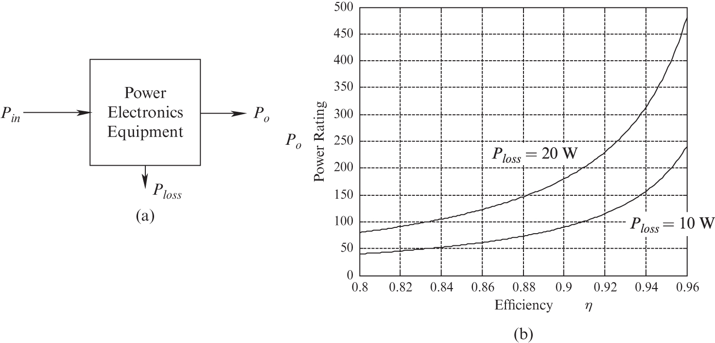
FIGURE 1.14 Power output capability as a function of efficiency
Equation 1.1 can be rewritten for the output power in terms of the efficiency and the power loss as:
Using Equation 1.2, the output power rating is plotted in Figure 1.14b, as a function of efficiency, for two values of Ploss.
In power electronics equipment, the cooling system is designed to transfer dissipated power, as heat, without allowing the internal temperatures to exceed certain limits. Therefore, for an equipment package designed to handle certain power loss dissipation, the plots in Figure 1.14b based on Equation 1.2 show that increasing the conversion efficiency from 84% to 94%, for example, increases the power output capability, same as the power rating, of that equipment by a factor of three. This could mean an increase in the power density, which is the power rating divided by the volume of the package, by approximately the same factor. This is further illustrated by Example 1.1 on the following page.
A power electronics package is designed to handle 200 W of power dissipation. Compare the two values of the output power capability if the conversion efficiency is increased from 89% to 94%.
Solution In this example, ![]() . Using Equation 1.2, at
. Using Equation 1.2, at ![]() ,
, ![]() , and at
, and at ![]() ,
, ![]() .
.
This example shows the importance of high energy conversion efficiency, where the power output capability and the power density (in watts per unit volume) of this package are nearly doubled by increasing the efficiency from 89% to 94%.
1.5 STRUCTURE OF POWER ELECTRONICS INTERFACE
By reviewing the role of power electronics in various applications discussed earlier, we can summarize that a power electronics interface is needed to efficiently control the transfer of power between DC-DC, DC-AC, and AC-AC systems. In general, the power is supplied by the utility, and hence, as depicted by the block diagram of Figure 1.15, the line-frequency AC is at one end. At the other end, one of the following is synthesized: adjustable magnitude DC, sinusoidal AC of adjustable frequency and amplitude, or high-frequency AC as in induction heating or systems using high-frequency transformers as an intermediate stage. Applications that do not require utility interconnection can be considered as the subset of the block diagram shown in Figure 1.15.
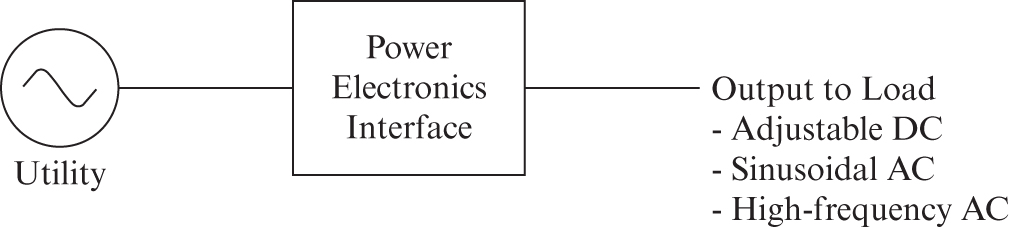
FIGURE 1.15 Block diagram of power electronic interface.
1.5.1 Voltage-Link Structure
To provide the needed functionality to the interface in Figure 1.15, the transistors and diodes, which can block voltage only of one polarity, have led to a commonly used voltage-link-structure, shown in Figure 1.16.

FIGURE 1.16 Voltage-link structure of power electronics interface.
This structure consists of two separate converters, one on the utility side and the other on the load side. The DC ports of these two converters are connected to each other with a parallel capacitor forming a DC-link, across which the voltage polarity does not reverse, thus allowing unipolar voltage-blocking transistors to be used within these converters.
In the structure of Figure 1.16, the capacitor in parallel with the two converters forms a DC voltage-link. Hence, it is called a voltage-link (or a voltage-source) structure. This structure is used in a very large power range, from a few tens of watts to several megawatts, even extending to hundreds of megawatts in utility applications. Therefore, we will mainly focus on this voltage-link structure in this book.
1.5.2 Current-Link Structure
At extremely high power levels, usually in utility-related applications, which we will discuss in the last two chapters in this book, it may be advantageous to use a current-link (also called current-source) structure, where, as shown in Figure 1.17, an inductor in series between the two converters acts as a current-link. These converters generally consist of thyristors, and the current in them, as discussed in Chapter 14, is “commutated” from one AC phase to another by means of the AC line voltages.

FIGURE 1.17 Current-link structure of power electronics interface.
1.5.3 Matrix Converters (Direct-Link Structure) [13]
Lately, in certain applications, a matrix converter structure, as shown in Figure 1.18 is being reevaluated, where theoretically, there is no energy storage element between the input and the output sides. Therefore, we can consider it to be a direct-link structure where input ports are connected to output ports by switches that can carry currents in both directions when on and block voltages of either polarity when off. A detailed discussion of matrix converters and their controls can be found in [13].
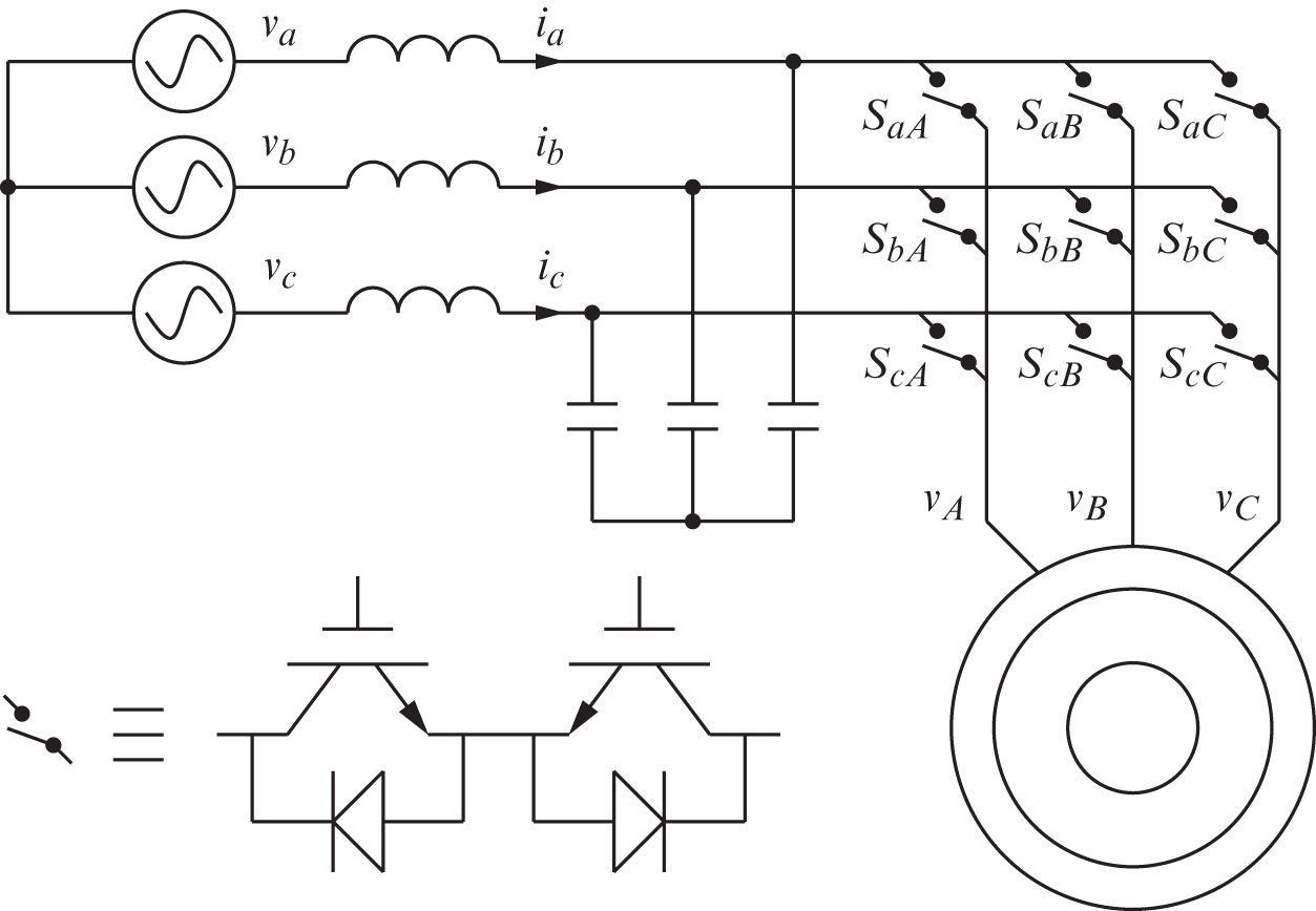
FIGURE 1.18 Matrix converter structure of power electronics interface. [13] / U.S department of energy / public domain.
1.6 VOLTAGE-LINK-STRUCTURE
In the voltage-link structure shown in Figure 1.16 and repeated in Figure 1.19, the role of the utility-side converter is to convert line-frequency utility voltages to an unregulated DC voltage. This can be done by a diode-rectifier circuit such as that discussed in basic electronics courses and also discussed in Chapter 5 of this textbook. However, the power quality concerns often lead to a different structure, discussed in Chapter 6. At present, we will focus our attention on the load-side converter in the voltage-link structure, where a DC voltage is applied as the input on one end, as shown in Figure 1.19.

FIGURE 1.19 Load-side converter in a voltage-source structure.
Applications dictate the functionality needed of the load-side converter. Based on the desired output of the converter, we can group these functionalities as follows:
Group 1
- Adjustable DC or a low-frequency sinusoidal AC output in
- – DC and AC motor drives
- – uninterruptible power supplies
- – regulated DC power supplies without electrical isolation
- – utility-related applications
Group 2
- High-frequency AC in
- – systems using high-frequency transformers as an intermediate stage
- – induction heating
- – regulated DC power supplies where the DC output voltage needs to be electrically isolated from the input, and the load-side converter internally produces high-frequency AC, which is passed through a high-frequency transformer and then rectified into DC.
We will discuss converters used in applications belonging to both groups. However, we will begin with converters for group-1 applications where the load-side voltages are DC or low-frequency AC.
1.6.1 Switch-Mode Conversion: Switching Power-Pole as the Building Block
Achieving high energy efficiency for applications belonging to either group mentioned above requires switch-mode conversion, where in contrast to linear power electronics, transistors (and diodes) are operated as switches, either on or off.
This switch-mode conversion can be explained by its basic building block, a switching power-pole A, as shown in Figure 1.20a. It effectively consists of a bi-positional switch, which forms a two-port: (1) a voltage-port across a capacitor with a voltage Vin that cannot change instantaneously, and (2) a current-port due to the series inductor through which the current cannot change instantaneously. For now, we will assume the switch is ideal with two positions: up or down, dictated by a switching signal qA, which takes on two values: 1 and 0, respectively. The practical aspects of implementing this bi-positional switch are what we will consider in the next chapter.

FIGURE 1.20 Switching power-pole as the building block in converters.
The bi-positional switch “chops” the input DC voltage Vin into a train of high-frequency voltage pulses, shown by vA waveform in Figure 1.20b, by switching up or down at a high repetition rate, called the switching frequency fs. Controlling the pulse width within a switching cycle allows control over the switching-cycle-averaged value of the pulsed output, and this pulse-width modulation forms the basis of synthesizing adjustable DC and low-frequency sinusoidal AC outputs, as described in the next section. High-frequency pulses are clearly needed in applications such as compact fluorescent lamps and induction heating and internally in DC power supplies where electrical isolation is achieved by means of a high-frequency transformer. A switch-mode converter consists of one or more such switching power-poles.
1.6.2 Pulse-Width Modulation (PWM) of the Switching Power-Pole (Constant fs)
For the applications in group 1, the objective of the switching power-pole redrawn in Figure 1.21a is to synthesize the output voltage such that its switching-cycle average is of the desired value: DC or AC that varies sinusoidally at a low frequency, compared to fs. Switching at a constant switching frequency fs produces a train of voltage pulses in Figure 1.21b that repeat with a constant switching time period Ts, equal to 1/fs.

FIGURE 1.21 PWM of the switching power-pole.
Within each switching cycle with the time period Ts (= 1/fs) in Figure 1.21b, the switching-cycle-averaged value ![]() of the waveform is controlled by the pulse width Tup (during which the switch is in the up position and vA equals Vin), as a ratio of Ts:
of the waveform is controlled by the pulse width Tup (during which the switch is in the up position and vA equals Vin), as a ratio of Ts:
where ![]() , which is the average of the qA waveform as shown in Figure 1.21b, is defined as the duty ratio of the switching power pole A, and the switching-cycle-averaged voltage is indicated by a “–” on top (the overbar symbol). The switching-cycle-averaged voltage and the switch duty ratio are expressed by lowercase letters since they may vary as functions of time. The control over the switching-cycle-averaged value of the output voltage is achieved by adjusting or modulating the pulse width, which later on will be referred to as pulse-width-modulation (PWM). This switching power-pole and the control of its output by PWM set the stage for switch-mode conversion with high energy efficiency.
, which is the average of the qA waveform as shown in Figure 1.21b, is defined as the duty ratio of the switching power pole A, and the switching-cycle-averaged voltage is indicated by a “–” on top (the overbar symbol). The switching-cycle-averaged voltage and the switch duty ratio are expressed by lowercase letters since they may vary as functions of time. The control over the switching-cycle-averaged value of the output voltage is achieved by adjusting or modulating the pulse width, which later on will be referred to as pulse-width-modulation (PWM). This switching power-pole and the control of its output by PWM set the stage for switch-mode conversion with high energy efficiency.
We should note that ![]() and dA in the above discussion are discrete quantities, and their values, calculated over a k-th switching cycle, for example, can be expressed as
and dA in the above discussion are discrete quantities, and their values, calculated over a k-th switching cycle, for example, can be expressed as ![]() and dA,k. However, in practical applications, the pulse-width Tup changes very slowly over many switching cycles, and hence we can consider them analog quantities as
and dA,k. However, in practical applications, the pulse-width Tup changes very slowly over many switching cycles, and hence we can consider them analog quantities as ![]() ðtÞ and dAðtÞ that are continuous functions of time. For simplicity, we may not show their time dependence explicitly.
ðtÞ and dAðtÞ that are continuous functions of time. For simplicity, we may not show their time dependence explicitly.
1.6.3 Switching Power-Pole in a Buck DC-DC Converter: An Example
As an example, we will consider the switching power-pole in a buck converter to step down the input DC voltage Vin, as shown in Figure 1.22a, where a capacitor is placed in parallel with the load to form a low-pass L-C filter with the inductor, to provide a smooth voltage to the load.

FIGURE 1.22 Switching power-pole in a buck converter.
In steady state, the DC (average) input to this L-C filter has no attenuation. Hence, the average output voltage Vo equals the switching-cycle average, ![]() , of the applied input voltage. Based on Equation 1.3, by controlling dA, the output voltage can be controlled in a range from Vin down to 0:
, of the applied input voltage. Based on Equation 1.3, by controlling dA, the output voltage can be controlled in a range from Vin down to 0:
In spite of the pulsating nature of the instantaneous output voltage ![]() , the series inductance at the current-port of the pole ensures that the current
, the series inductance at the current-port of the pole ensures that the current ![]() remains relatively smooth, as shown in Figure 1.22b.
remains relatively smooth, as shown in Figure 1.22b.
In the converter of Figure 1.22a, the input voltage ![]() . The output voltage
. The output voltage ![]() . Calculate the duty ratio
. Calculate the duty ratio ![]() and the pulse width Tup, if the switching frequency fs = 200 kHz.
and the pulse width Tup, if the switching frequency fs = 200 kHz.
Solution ![]() . Using Equation 1.4,
. Using Equation 1.4, ![]() and
and ![]() .
.
Therefore, as shown in Figure 1.23, ![]() .
.

FIGURE 1.23 Waveforms in the converter of Example 1.2.
1.6.3.1 Realizing the Bi-Positional Switch in a Buck Converter
As shown in Figure 1.24a, the bi-positional switch in the power pole can be realized by using a transistor and a diode. When the transistor is gated on (through a gate circuitry, discussed in the next chapter, by a switching signal qA = 1), it carries the inductor current, and the diode is reversed biased, as shown in Figure 1.24b. When the transistor is switched off (qA = 0), as shown in Figure 1.24c, the inductor current “freewheels” through the diode until the next switching cycle when the transistor is turned back on. The switching waveforms, shown earlier in Figure 1.22b, are discussed in detail in Chapter 3.

FIGURE 1.24 Transistor and diode forming a switching power-pole in a buck converter.
In the switch-mode circuit of Figure 1.22a, the higher the switching frequency, that is, the frequency of the pulses in the vA(t) waveform, the smaller the values needed for the low-pass L-C filter. On the other hand, higher switching frequency results in higher switching losses in the bi-positional switch, which is the subject of the next chapter. Therefore, an appropriate switching frequency must be selected, keeping these trade-offs in mind.
1.7 RECENT ADVANCES IN SOLID-STATE DEVICES BASED ON WIDE BANDGAP (WBG) MATERIALS
There have been significant advances in the wide bandgap (WBG) materials that have made WBG devices such as GaN- and SiC-based diodes and MOSFETs available at reasonable prices for power electronics applications. These include SiC-MOSFETs with voltage-blocking capabilities as high as 1.7 kV.
In comparison to these WBG devices, the silicon power device technology is mature, and only minor evolutionary improvements are likely. These devices are limited to junction temperatures < 150–200 °C. However, power electronics applications are extending to ever higher voltages, higher frequencies, higher temperatures, and higher efficiencies simultaneously. This makes the use of Si-based devices in future applications increasingly difficult and expensive.
WBG devices offer a potential solution where they are especially better for higher voltages (> 1000 V) as well as in low-voltage applications below 600 volts or so. They are faster, have lower losses, and higher operating temperatures to minimize the thermal management systems.
WBG devices operate by the same physical mechanisms as Si devices and have similar geometries. Their better performance is due to superior material properties. The WBG materials of interest are gallium nitride (GaN) and silicon carbide (SiC). The WBG devices are fundamentally superior to Si devices for the basic reason of 10 times larger breakdown field strength of the WBG materials that enable faster switching with lower losses, higher temperature operation, and higher thermal conductivity.
A variety of SiC-devices are commercially available, and SiC MOSFETs and diodes will dominate power electronic applications above 1000 V. Similarly, GaN-based diodes and MOSFETs will dominate power electronic applications below 600 V. Their applications are shown in Figure 1.25 as functions of the operating frequencies and power levels.

FIGURE 1.25 Applications of SiC- and GaN-based devices.
[Source: Graph used under kind permission of Infineon Technologies AG] [14]; https://www.infineon.com/cms/en/product/technology/wide-bandgap-semiconductors-sic-gan.
Further details on WBGs can be found in [13].
1.8 USE OF SIMULATION AND HARDWARE PROTOTYPING
Throughout this book, modeling tools are used to facilitate discussion and provide an in-depth understanding of the concepts in power electronics. LTspice and Sciamble™ Workbench [15] are computer simulation tools used to demonstrate all topics in this book.
LTspice is a widely used SPICE-based circuit simulator. Sciamble™ Workbench is a mathematical simulation tool developed at the University of Minnesota. All examples and key concepts explained in this book are also simulated using both LTspice and Workbench, and the results are provided on the accompanying website.
A noteworthy motivation for using Sciamble™ Workbench is its seamless transition between mathematical simulation and hardware prototyping modes. Hardware prototyping simplifies the development of a real-time controller enabling rapid laboratory experimentation of concepts covered in this book. Real-world experimentation enables a more in-depth and practical understanding of the contents of this book. Sciamble™’s power electronics hardware kit is used for laboratory implementation of all the topics in this book.
All the simulation files using both LTspice and Sciamble™ Workbench, as well as the manual for laboratory implementation using Workbench, are available on the accompanying website.
REFERENCES
- 1. N. Mohan, T.M. Undeland, and W.P. Robbins, Power Electronics: Converters, Applications and Design, 3rd Edition (New York: John Wiley & Sons, 2003).
- 2. N. Mohan and R.J. Ferraro, “Techniques for Energy Conservation in AC Motor Driven Systems,” EPRI-Report EM-2037, Project 1201 1213, September 1981.
- 3. N. Mohan and J. Ramsey, “Comparative Study of Adjustable-Speed Drives for Heat Pumps,” EPRI-Report EM-4704, Project 2033–4, August 1986.
- 4. Improving Motor and Drive System Performance: A Sourcebook for Industry, Industrial Technologies Program (ITP) (Book), US Department of Energy (energy.gov). https://www1.eere.energy.gov/manufacturing/tech_assistance/pdfs/motor.pdf.
- 5. “Significant Progress in Lithium-air Battery Development,” ScienceDaily. https://www.sciencedaily.com/releases/2021/05/210506104801.htm.
- 6. “Progress in Hydrogen and Fuel Cells.” US Department of Energy. https://www.energy.gov/eere/fuelcells/articles/progress-hydrogen-and-fuel-cells.
- 7. “Alternative Fuels Data Center: Emissions from Electric Vehicles,” US Department of Energy. https://afdc.energy.gov/vehicles/electric_emissions.html.
- 8. “Toyota Electric Vehicles.” https://www.toyota.com/electrified.
- 9. “Alternative Fuels Data Center: Maps and Data—Average Fuel Economy by Major Vehicle Category,” US Department of Energy. https://afdc.energy.gov/data/10310.
- 10. “Car Emissions and Global Warming,” Union of Concerned Scientists (Ucsusa.org). https://www.ucsusa.org/resources/car-emissions-global-warming.
- 11. “Power Electronics in Automotive Applications,” Elprocus. https://www.elprocus.com/power-electronics-in-automotive-applications.
- 12. The American Clean Power Association. cleanpower.org.
- 13. N. Mohan, W. Robins, T. Undeland, and S. Raju, Power Electronics for Grid-Integration of Renewables: Analysis, Simulations and Hardware Lab (New York: John Wiley & Sons, 2023).
- 14. “Wide Bandgap Semiconductors (SiC/GaN),” Infineon. https://www.infineon.com/cms/en/product/technology/wide-bandgap-semiconductors-sic-gan.
- 15. Sciamble™ Workbench platform. https://sciamble.com.
PROBLEMS
Applications and Energy Conservation
- 1.1 A US Department of Energy report [4] estimates that over 122 billion kWh/year can be saved in the manufacturing sector in the United States by using mature and cost-effective conservation technologies. Calculate (a) how many 1,100-MW generating plants are needed to operate constantly to supply this wasted energy, and (b) the annual savings in dollars if the cost of electricity is 0.12 cents/kWh.
- 1.2 In a process, a blower is used with the flow-rate profile shown in Figure P1.1a.

FIGURE P1-1 Flowrate profile.
Using the information in Figure P1.1b, estimate the percentage reduction in power consumption resulting from using an adjustable-speed drive rather than a system with (a) an outlet damper and (b) an inlet vane.
- 1.3 In a system, if the system size is based on power dissipation capacity, calculate the improvement in the power density if the efficiency is increased from 87% to 95%.
- 1.4 The electricity generation in the United States is approximately
 MW-hrs. Figure 1.7 shows that 16% of that is used for heating, ventilating, and air conditioning. As much as 30% of the energy can be saved in such systems by using adjustable-speed drives. On this basis, calculate the savings in energy per year and relate that to 1,100-MW generating plants needed to operate constantly to supply this wasted energy.
 - 1.5 The total amount of electricity that could potentially be generated from wind in the United States has been estimated at
 MW-hrs annually. If one-tenth of this potential is developed, estimate the number of 1.5 MW windmills that would be required, assuming that on average a windmill produces only 30% of the energy that it is capable of.
 - 1.6 In Problem 1.5, if each 1.5 MW windmill has all its output power flowing through the power electronics interface, estimate the total rating of these interfaces in MW.
- 1.7 As the pie chart of Figure 1.7 shows, lighting in the United States consumes 19% of the generated electricity. LEDs consume power one-sixth of that consumed by the incandescent lamps for the same light output. Electricity generation in the United States is approximately
 MW-hrs. Based on this information, estimate the savings in MW-hrs annually, assuming that all lighting at present is by incandescent lamps, which are to be replaced by LEDs.
 - 1.8 An electric-hybrid vehicle offers 52 miles per gallon in mixed (city and highway) driving conditions according to the US Environmental Protection Agency. This is in comparison to the gas mileage of 22.1 miles per gallon for an average passenger car in the United States, with an average of 11,766 miles driven per year. Calculate the savings in terms of barrels of oil per automobile annually if a conventional car is replaced by an electric-hybrid vehicle. In calculating this, assume that a barrel of oil that contains 42 gallons yields approximately 20 gallons of gasoline.
- 1.9 We can project that there are 150 million cars in the United States. Using the results of Problem 1.8, calculate the total annual reduction of carbon into the atmosphere if the consumption of each gallon of gasoline releases approximately 5 pounds of carbon.
- 1.10 Relate the savings of barrels of oil annually, as calculated in Problem 1.9, to the imported oil if the United States imports approximately 35,000 million barrels of crude oil per year.
- 1.11 Fuel-cell systems that also utilize the heat produced can achieve efficiencies approaching 80%, more than double of the gas-turbine-based electrical generation. Assume that 20 million households produce an average of 5 kW. Calculate the percentage of electricity generated by these fuel-cell systems compared to the annual electricity generation in the United States of
 MW-hrs.
 - 1.12 Induction cooking based on power electronics is estimated to be 80% efficient compared to 55% for conventional electric cooking. If an average home consumes 2 kW-hrs daily using conventional electric cooking, and that 20 million households switch to induction cooking in the United States, calculate the annual savings in electricity usage.
- 1.13 Assume the average energy density of sunlight to be 800 W/m2 and the overall photovoltaic system efficiency to be 10%. Calculate the land area covered with photovoltaic cells needed to produce 1,000 MW, the size of a typical large central power plant.
- 1.14 In Problem 1.13, the solar cells are distributed on top of roofs, each in an area of 40 m2. Calculate the number of homes needed to produce the same power.
- 1.15 Describe the role of power electronics in harnessing onshore and offshore wind energy.
- 1.16 Describe the role of power electronics in photovoltaic systems to harness solar energy.
- 1.17 Describe the role of power electronics in battery storage and fuel-cell systems.
- 1.18 Describe the role of power electronics in electric vehicles, hybrid-electric vehicles, and plug-in hybrid-electric vehicles.
- 1.19 Describe the role of power electronics in transportation systems by means of high-speed rails.
- 1.20 Describe the role of power electronics for energy conservation in lighting using LEDs.
- 1.21 Describe the role of power electronics for energy conservation in heat pumps and air conditioners.
- 1.22 Describe the role of power electronics in transmitting electricity by means of high-voltage DC (HVDC) transmission.
PWM of the Switching Power-Pole
- 1.23 In a buck converter, the >input voltage Vin = 12 V. The output voltage Vo is required to be 9 V. The switching frequency fs = 400 kHz. Assuming an ideal switching power-pole, calculate the pulse width Tup of the switching signal and the duty ratio dA of the power pole.
- 1.24 In the buck converter of Problem 1.23, assume the current through the inductor to be ripple-free with a value of 1.5 A (the ripple in this current is discussed later in Chapter 3). Draw the waveforms of the voltage vA at the current-port and the input current iin at the voltage-port.
- 1.25 Using the input-output specifications given in Problem 1.23, calculate the maximum energy efficiency expected of a linear regulator where the excess input voltage is dropped across a transistor, that functions as a controllable resistor and is placed in series between the input and the output.
Simulation Problems
- 1.26 In the circuit diagram of the buck converter in Figure 1.22a, the low-pass filter has the following values: L = 5 μH and C = 100 μF. The output load resistance is R = 0.5 Ω. The input voltage vA is a pulse waveform between 0 and 10 volts, with a pulse width of 0.75 μs and a frequency fs = 100 kHz.
- Plot the input voltage vA and the output voltage vo for the last 10 switching cycles after vo waveform has reached its steady state.
- How does Vo relate to
 (the average of vA)?
 - What is the ratio of the switching frequency to the L-C resonance frequency? By means of Fourier analysis, compute the attenuation of the fundamental-frequency component in the input voltage by the filter at the switching frequency?
- 1.27 In Problem 1.26, plot the gain of the transfer function
 in dB, as a function of frequency. Does the frequency at which the transfer-function gain is peaking coincide with the L-C resonance frequency? Calculate the attenuation of the fundamental-frequency component by the filter. How does it compare with that obtained by the Fourier analysis in Problem 1.26c?