
![]()
Logistic Regression
In previous chapters, we covered correlation and linear regression modeling in detail. If you look to quantify the relationship between two variables, you use the correlation coefficient. For example, you can quantify the relation between salary and expenses using correlation. If you needed to predict a response variable based upon some other item, you could use linear regression modeling, provided the relationship is linear. For example, if you want to predict exactly what a person’s expenses will be when his salary is $10,000, you can use linear regression modeling, provided the expense and salary fit on a straight-line graph. In some cases, this relationship is not actually linear, but you can make it linear by applying some simple mathematical transformations; still, you can use linear regression modeling.
Is linear regression modeling the solution for all real-life prediction problems? Or do you need to apply different techniques in some cases? Let’s explore these questions using a simple example.
Predicting Ice-Cream Sales: Example
Table 11-1 shows a snapshot of a table that contains the ice-cream sales data for an ice-cream shop. For now, you are recording just two variables: the age of the customer and whether she buys ice cream. The data set has an indicator variable called buy_ind, which takes a value of 0 if a customer buys ice cream and a value of 1 if not. You are asked to predict ice-cream sales (in other words, the buy_ind variable) using age as an independent variable.
Table 11-1. Ice-Cream Sales Data
|
Age |
buy_ind |
|---|---|
|
6 |
0 |
|
25 |
0 |
|
32 |
1 |
|
44 |
1 |
|
34 |
1 |
|
43 |
1 |
|
72 |
1 |
|
67 |
0 |
|
58 |
1 |
|
. |
. |
|
. |
. |
|
58 |
1 |
The data set has just two variables: buy_ind and Age. The following is the SAS code for importing the data and building a simple linear regression line for the response variable:
/* Importing ice cream sales data*/
PROC IMPORT OUT= WORK.ice_cream_sales
            DATAFILE= "C:UsersVENKATGoogle DriveTrainingBooksConte nt8.
Logistic RegressionData Logistic RegressionIceCream_sales.csv"
            DBMS=CSV REPLACE;
     GETNAMES=YES;
     DATAROW=2;
RUN;

/* Fitting a simple regression line to predict buy_ind */
proc reg data=ice_cream_sales;
model buy_ind=age;
run;
Table 11-2 shows the output of the previous code.
Table 11-2. Output of PROC REG on Ice-Cream Sales Data

The following are the observations and inferences for the output in Table 11-2:
- There are a total of 50 observations used for building this model.
- The P-value of the F-testis less than 5 percent, which suggests that the overall model is significant.
- The R-squared value is on the lower side, which shows that the model is not a good fit. In other words, you can’t expect it to deliver respectable predictions.
- The Age variable seems to significantly impact buying. This has been indicated by the P-value of T-test for Age.
- To summarize, you can’t use this model for your predictions. It is not a good fit.
By this time, having learned so much about regression, the model fitting for the ice-cream sales data may appear to be a routine exercise. You can easily conclude that the fit is not good for the data. The variable Age can’t explain much of the variation in buying, which means whether a customer buys the ice-cream or not can’t be estimated simply by the variable Age. In other words, simply by knowing a customer’s specific age, you can’t tell anything about ice-cream sales.
On second thought, when you take a close look at the data, you can easily observe a pattern in it. You can see that when customer is younger, the buy_ind variable is 0 most of the time, and when customer is older, buy_ind is 1 most of the time. This shows that older people are not buying ice cream. A scatterplot between the two variables reiterates the same (Figure 11-1).
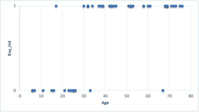
Figure 11-1. Scatterplot on ice-cream sales data
Figure 11-1 shows that almost all customers younger than 30 have bought ice cream, and almost all the customers older than 30 haven’t. The data has some apparent pattern, but you are not able to capture it using the linear regression models. Maybe a linear regression line is not a good fit for this data. See Figures 11-2 and 11-3.

Figure 11-2. A straight line is not a good fit for the ice-cream sales data

Figure 11-3. A straight line is not a good fit for the ice-cream sales data
No matter what optimization technique you apply, you can’t come up with a straight line that will pass through the core of the data. If you recall the regression assumptions from regression in Chapter 9, you will realize that when the relation between the dependent (buy_ind) and independent (Age) variables is not linear, you can’t apply a linear regression model. This is the case here.
If the relation between x and x is nonlinear and if it cannot be converted to a linear relationship by applying mathematical transformations, then you need to fit the best applicable nonlinear curve. Anything other than a straight-line relationship is termed nonlinear. Since you could not fit a linear regression line to the ice-cream sales data, let’s see if you can fit a nonlinear curve. Figures 11-4 to 11-8 are some examples of nonlinear expressions.

Figure 11-4. Log(x)

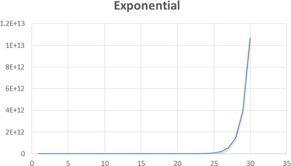
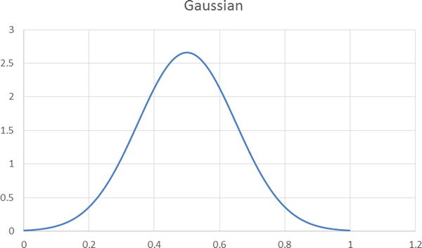

Figure 11-8. Logit function
Out of all nonlinear functions given, you can see that a logistic curve looks like a perfect fit for this data, where all the Y values are either 0 or 1. A logistic curve has very long tails around 0 and 1, and values other than 0 and 1 are minimal. Hence, you can choose the logistic regression for the type of data, where you have only two outcomes (0 and 1). Please note that the theory behind choosing a logistic line is a little complicated, and the logic given here is only a simplified version.
Because the ice-cream sales data is all about 0s and 1s, let’s try to fit a logistic regression curve. Figure 11-9 is an imaginary logistic curve of the data.

Figure 11-9. An imaginary logistic curve through the ice-cream sales data
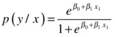
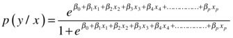
You have the straight equation ![]() for linear regression. In a similar fashion, you have an equation for the logistic line as well.
for linear regression. In a similar fashion, you have an equation for the logistic line as well.

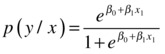
The logistic function, explained by the earlier equation, is never less than 0 and never greater than 1. The maximum value is 1; ![]() tends to give very high values, or it tends to reach infinity. For example, if the numerator is 1,000,000, then the denominator will take a value of 1,000,001. In such a case, the probability is almost 1. The lower limit is 0; imagine a numerator of 0.0000000001. The denominator is 1.0000000001, and then the probability value is almost 0.
tends to give very high values, or it tends to reach infinity. For example, if the numerator is 1,000,000, then the denominator will take a value of 1,000,001. In such a case, the probability is almost 1. The lower limit is 0; imagine a numerator of 0.0000000001. The denominator is 1.0000000001, and then the probability value is almost 0.
Please note that you are not trying to predict Y, but you are trying to predict the probability of Y=0 or Y=1. Since Y takes just two values, there is hardly any variation in Y. So, it makes more sense to predict the probabilities rather than direct values.
Logistic regression may be a perfect choice when you have just two outcomes in your response variable. You encounter only two outcomes situations in many cases like these: yes versus no in response to a question, win versus loss in a game, buy versus no buy in customer sales, response versus no response in cold calling, click versus no click in web analytics, default versus no default in credit risk analysis, satisfied versus not satisfied in survey analytics, and so on. It is not possible to predict these categorical outcomes using linear regression because it expects numeric dependent variables.
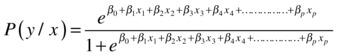
Here is the logistic line equation discussed in the previous section. It’s for a single independent variable.
Here is the logistic line equation for multiple independent variables:

The previous equations can be written in logarithmic teams as follows.

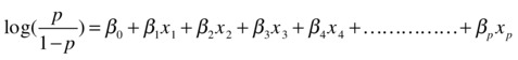
 is called the log odds probability. Here you are trying to fit a line that predicts the log odds of Y rather than its direct values. In the same way as the least squares methodology is used to fit linear regression coefficients (please refer to Chapter 9), the maximum likelihood estimation (MLE) method is used to find the beta coefficients if you have a logistic regression line. We will not get into the details of the MLE method, but you can consider it an optimization technique that is used to find the coefficients in a logistic regression line.
An analyst has to first sense the applicability of logistic regression by looking at the dependent variable and applying the logistic regression procedure in SAS instead of the usual linear regression. You used the PROC REG procedure for linear regression. For finding out the beta coefficients in the case of logistic regression, you will use the PROC LOGISTIC procedure from SAS.
You have discovered that linear regression is not the right regression line to fit the ice-cream sales case. You also discovered that a logistic regression line would be a better fit. Now you will create a logistic regression model using SAS.
The following is the SAS code to fit the desired logistic regression line:
Proc logistic data=ice_cream_sales;
model buy_ind=age;
run;
Here is an explanation of the code:
- PROC LOGISTIC: This calls the logistic regression line procedure in SAS.
- Data: This indicates the ice_cream_sales data set.
- Model: This is similar to a linear regression line. The dependent variable is on the left side of the equal sign, and a list of independent variables is on the right side. Multiple independent variables (if available) are separated by a single space between them.
The previous code tries to fit a logistic regression line to the ice-cream sales data, which means that you are trying to estimate the beta coefficients in the logistic regression equation, given here:
This code generates the output shown in Table 11-3.
Table 11-3. Output of PROC LOGISTIC on Ice-Cream Sales Data
|
The SAS System | |
|---|---|
|
The LOGISTIC Procedure | |
|
Model Information | |
|
Data Set |
WORK.ICE_CREAM_SALES |
|
Response Variable |
buy_ind |
|
Number of Response Levels |
2 |
|
Model |
binary logit |
|
Optimization Technique |
Fisher’s scoring |
|
Number of Observations Read |
50 |
|
Number of Observations Used |
50 |
Response Profile | ||
|---|---|---|
Ordered Value |
buy_ind |
Total Frequency |
|
1 |
0 |
15 |
|
2 |
1 |
35 |
| Probabilitymodeledisbuy_ind=‘0’. | ||
|
Model Convergence Status |
|
Convergence criterion (GCONV=1E-8) satisfied. |
|
Model Fit Statistics | ||
|---|---|---|
Criterion |
Intercept Only |
Intercept and Covariates |
|
AIC |
63.086 |
36.114 |
|
SC |
64.998 |
39.938 |
|
-2 Log L |
61.086 |
32.114 |


SAS Logistic Regression Output Explanation
The output has several measures and tables. The following sections explain.
Output Part 1: Response Variable Summary
Table 11-4 shows the LOGISTIC procedure.
Table 11-4. Model Information, Output of PROC LOGISTIC
|
Model Information | |
|---|---|
|
Data Set |
WORK.ICE_CREAM_SALES |
|
Response Variable |
buy_ind |
|
Number of Response Levels |
2 |
|
Model |
binary logit |
|
Optimization Technique |
Fisher’s scoring |
Here is an explanation of Table 11-4:
- Data set: This is the data source.
- Response variable: This is the dependent variable or the Y variable, the buying indicator in this example.
- Number of response levels: This is the number of levels in the dependent variable (mostly Yes/No); it’s 1 or 0 in this example.
- Model: This is the binary logistic regression; it’s the same as binary logit.
- Optimization technique: Which optimization technique is used to find the regression coefficients? SAS chooses the most appropriate technique.
Now consider more tables from the output in Table 11-5.
Table 11-5. Output Tables of PROC LOGISTIC
|
Number of Observations Read |
50 |
|---|---|
|
Number of Observations Used |
50 |
|
Response Profile | |||
|
Ordered Value |
buy_ind |
Total Frequency | |
|---|---|---|---|
|
1 |
0 |
15 | |
|
2 |
1 |
35 |
Probability modeled is buy_ind=‘0’. |
Here is an explanation of Table 11-5:
- Number of observations read: This is the count of observations read from the data set.
- Number of observations used: This is the number of observations used for creating the model. There are no missing values or default values in the data. If there are missing values, SAS will give a count of those missing values separately.
- Response profile ordered values: This is how SAS ordered the values that you supplied. It considered the 0 category the first level and the 1 category the second level.
- Probability modeled is buy_ind=‘0’: The logistic regression will finally give the probability of Y, which can take a value of 0 or 1. In this output, SAS is informing you that the model is built for 0; in other words, the output probability will be given for the occurrence of Y being 0. By default SAS builds the model for smaller values. It doesn’t really matter when you have only two levels. If the probability of 0 is 65 percent, then the probability of 1 will obviously be 35 percent. You can use the descending option (refer to the case study later in this chapter, where SAS code with this option has been used) to directly model for the higher-order value. As per the output, in the ice-cream sales example, the model is built for the probability of Y being 0, which means a buy decision.
- Total frequency: This is the frequency of each category in a dependent variable.
Output Part 2: Model Fit Summary
In output part 2, we discuss the model convergence status and the model fit statistics. Refer to Table 11-6.
Table 11-6. Model Fit Summary, the Output Tables of PROC LOGISTIC
|
Model Convergence Status |
|---|
|
Convergence criterion (GCONV=1E-8) satisfied. |
|
Model Fit Statistics | ||
|
Criterion |
Intercept Only |
Intercept and Covariates |
|---|---|---|
|
AIC |
63.086 |
36.114 |
|
SC |
64.998 |
39.938 |
|
-2 Log L |
61.086 |
32.114 |
Here is an explanation of the Table 11-6:
- Model convergence status: This is related to your model’s optimization convergence and precision. A detailed explanation on this is beyond the scope for this book.
- Model fit statistics:
- AIC: Akaike Information Criterion is a measure that is used to compare two models so as to pick the best one. Generally, a model with less AIC is desired. A stand-alone AIC value is not of much significance, so you can ignore it for now.
- SC: Schwarz Criterion is similar to AIC, used for comparing two models. AIC and SC values will be less for models that have a fewer number of predictor variables and high accuracy in line fitting. For example, if you are comparing two models to find which one is better, you should go for the model that has minimum AIC and SBC. Generally, AIC and SC are less for the models, which have high accuracy with fewer predictor variables.
Output Part 3: Test for Regression Coefficients
In part 3, you are testing the global null hypothesis for beta = 0. Table 11-7 shows the test results for the null hypothesis (that the coefficients of all the independent variables are equal to zero) versus the alternative hypothesis (that at least one of the confidents is nonzero). In other words, you are testing whether all the independent (X) variables are insignificant versus at least one of them is significant.
H0: ![]()
vs
H1: ![]()
Table 11-7. Testing Global Null Hypothesis, the Output Tables of PROC LOGISTIC
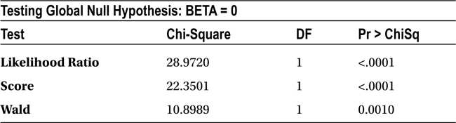
All these three tests (Likelihood, Score, and Wald) are testing the previous hypothesis only. If all the tests show that the P-value (Pr > ChiSq) is greater than 5 percent, then there is not much evidence to reject the null hypothesis. This means there is not even a single variable that has a significant impact (on Y). If in any of the tests the P-value is less than 5 percent, then there is at least one variable that has a significant impact on the dependent variable. Mostly all three tests show the same result. Here in this example, the Chi-square tests show that the null hypothesis is rejected. This means there is at least one independent variable whose coefficient is not equal to zero.
Output Part 4: The Beta Coefficients and Odds Ratio
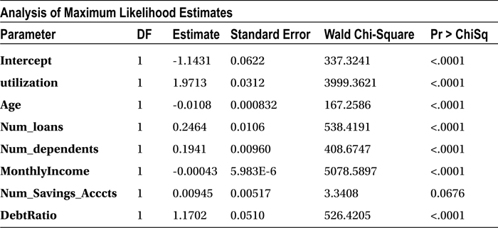
The coefficients, the regression parameters, or the beta values of the independent variable are given in Table 11-8.
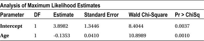
Table 11-8. Analysis of Maximum Likelihood Estimates, the Output Tables of PROC LOGISTIC
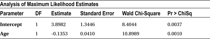
The table (Analysis of Maximum Likelihood Estimates) shows the MLE estimates for the independent variable coefficients, as given by the following equation:

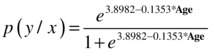
The value of β0 is 3.8982, and the value of β1 is -0.1353.
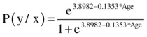
The following is the logistic regression line equation based on the estimates given by SAS:
![]()
![]()
You can substitute the values of age in this equation to find the probability of buying for each customer.
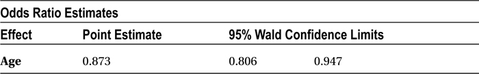
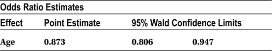
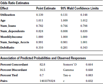
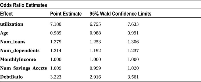
The odds ratio estimates (Table 11-9) are a little different from the previous estimates. These estimates are used to see the exact impact of each individual variable on the odds of the positive outcome of the model. For instance, you are predicting the probability of buying ice cream in this example. The odds ratio estimates tell you what the impact of age is on the odds of buying (in other words, the chances of buying). What is the change in the odds when there is a unit change in the independent variable? In this model, the change in odds is 0.873 whenever there is a unit change in the age.
Table 11-9. Odds Ratio Estimates, the Output Tables of PROC LOGISTIC
The following is the regression line for ice-cream sales data; you substitute the age to find the predicted probability of buying:

For example, when the age is 6, the probability of buying is 95.6 percent, and the probability of not buying is 4.3 percent. The odds of buying over not buying are 95 percent/5 percent, that is, 21.8981.
When the age is increased by one unit, such as increased to 7 from 6, the probability of buying is 95.03 percent and not buying is 4.968 percent. The odds of buying over not buying are 95.03 percent/4.968 percent, that is, 19.12698.
When you changed the age by one unit, from 6 to 7, the odds also changed, from 21.8981 to 19.12698. The odds ratio is 0.8734 (odds of buying over not buying [age=7]/the odds of buying over not buying [age=6]), which is the same as given in the odds ratio estimate table in SAS. The odds ratio estimate gives you the estimate of exact change in the odds when there is a unit change in the independent variable. Table 11-10 illustrates the same.
Table 11-10. Change in odds with unit change age

From Table 11-10, you can see that the odds ratio is exactly 0.8734 whenever there is a change of 1 unit in the independent variable, such as the age.
Output Part 5: Validation Statistics
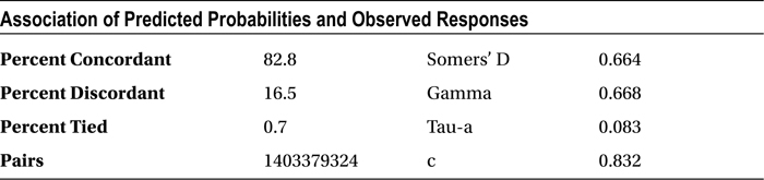
Table 11-11 is an important table because you can use it for validating the model. This gives you an idea about misclassification errors and the effectiveness of the model. A higher percent of concordance is always desired. Somers’ D, Gamma, Tau-a, and C are derived from misclassification versus classification only.
Classifying 0 as 0 or giving a higher probability to 0 when the actual dependent variable value is 0 is classification without error. If the model is classifying 0 as 1 and 1 as 0 or giving a higher probability to 0 when the actual dependent value is 1, or vice versa, it is misclassification. We will explain classification and misclassification in detail in the “Goodness of Fit for Logistic Regression” section.
Table 11-11. Association of Predicted Probabilities and Observed Responses, the Output Tables of PROC LOGISTIC

Individual Impact of Independent Variables
In linear regression models, you used the P-value to check whether an independent variable has a significant impact on a dependent variable. The beta coefficients in linear regression follow T-distribution, so you did a T-test to see the impact of each variable. Here in logistic regression, the beta coefficients follow the Chi-square distribution. So, the probability value (P-value) of the Chi-square test tells you about the impact of the independent variables in logistic regression models.
A Chi-square test in logistic regression tests the hypotheses here:
H0: The independent variable has no significant impact on the dependent variable.
H1: The independent variable has significant impact on the dependent variable.
You will look at the P-value of the Chi-square test to make a decision on acceptance or rejection of the hypothesis.
- If the P-value of the Chi-square test is less than 5 percent, you reject the null hypotheses; you reject the null hypothesis that the variable has no significant impact on the dependent variable. This means that the variable has some significant impact; hence, you keep it in the model.
- If the P-value of the Chi-square test is greater than 5 percent, then there is not enough evidence to reject the null hypotheses. So, you accept the null hypothesis that the variable has no significant impact on the dependent variable; hence, you drop it from the model. Dropping such insignificant variables from the model will have no influence on model accuracy.
You can take a look at the Wald Chi-square value when you are comparing two independent variables to decide which variable has a greater impact. If Wald Chi-square value is high, then the P-value is low. For example, if you are comparing the impact of two independent variables such as income and number of dependents on the response variable, then the variable with the higher Wald Chi-square value will be chosen because it has a higher impact on the dependent variable (or response variable).
Table 11-12 is the Chi-square test table from the ice-cream sales example.
Table 11-12. Chi-square Test, the Output Tables of PROC LOGISTIC

- H0: Age has no significant impact on ice-cream purchase.
- H1: Age has a significant impact on ice-cream purchase
The P-value for the Age variable is 0.0010, which is less than 0.05 (5 percent). So, you can reject the null hypothesis, which would mean that age has a significant impact on ice-cream purchase. Logistic regression:independent variables
Goodness of Fit for Logistic Regression
In this section, we will discuss the Chi-square test in detail, and concordance.
The Chi-square value and the associated Chi-square test is a basic measure of goodness of fit in logistic regression. The Chi-square test is used for testing the null hypothesis that all the independent variables’ regression coefficients are zero versus at least one of the independent variables is significant. The Chi-square test is similar to F-test in linear regression.
H0 :
 .
.- This is same as
 and
and  and
and  and
and  .
. - This means that the overall model is insignificant or it has no explanatory power.
H1 :
 .
.- This is same as at least one
 .
. - This means that at least one variable is significant, or the model has some explanatory power.
If the P-value of the Chi-square test is greater than 5 percent, then the model is at risk. If the P-value is more than 5 percent, then you have to accept the null hypothesis, which means the overall model is insignificant. There is no point in proceeding further, and none of the independent variables has significant impact on the dependent variable. It forces you to collect more data and look for more impactful independent variables. In the SAS output, you see three Chi-square tests—Likelihood Ratio, Score, and Wald—all of them for the same purpose. Generally, all these tests show the same result.
As discussed earlier, the concordance measure gives you an estimate of accuracy or the goodness of fit of your logistic regression model. You will consider an example in this section to understand concordance and discordance.
Imagine a simple data set where there are just 10 observations. Five records of the dependent variable take a value of 1; the other five are at 0. After building the model, you will determine the predicted probability of the dependent variable for each record. It looks like Table 11-13.
Table 11-13. Predicted Probability of Dependent Variable
|
DEPENDENT VARIABLE |
PREDICTED PROBABILITY |
|---|---|
|
0 |
P1 |
|
0 |
P2 |
|
0 |
P3 |
|
0 |
P4 |
|
0 |
P5 |
|
1 |
P6 |
|
1 |
P7 |
|
1 |
P8 |
|
1 |
P9 |
|
1 |
P10 |
You can make as many as 25 pairs using five 0s and five 1s along with their corresponding probabilities.
(0 P1 – 1 P6), (0 P1 – 1 P7), (0 P1 – 1 P8), (0 P1 – 1 P9), (0 P1 – 1 P10)
(0 P2 – 1 P6), (0 P2 – 1 P7), (0 P2 – 1 P8), (0 P2 – 1 P9), (0 P2 – 1 P10)
(0 P3 – 1 P6), (0 P3 – 1 P7), (0 P3 – 1 P8), (0 P3 – 1 P9), (0 P3 – 1 P10)
(0 P4 – 1 P6), (0 P4 – 1 P7), (0 P4 – 1 P8), (0 P4 – 1 P9), (0 P4 – 1 P10)
(0 P5 – 1 P6), (0 P5 – 1 P7), (0 P5 – 1 P8), (0 P5– 1 P9), (0 P5 – 1 P10)
Take the first pair (0 P1 – 1 P6). If you built a model to predict the value 0, then P1 should be higher than P6. A good model should give higher probabilities to zero and lower probabilities to 1. Hence, P1 should be greater than P6 in the first pair, P1 should be greater than P7 in the second pair, and P5 should be greater than P10 in the last pair. This accurate classification is called concordance. Percent concordance is the percentage of concordance cases in all possible pairs. The higher the percent concordance, the higher the accuracy of the model.
If in the first pair (0 P1 – 1 P6) if P1 is less than P6, then it is not a good sign. You built a model to predict zero, and the model is finally predicting higher probabilities for 1 and lower probability for 0. This misclassification is called discordance. The percentage of discordant pairs in overall (all possible pairs) is called percent discordance.
For example, take the data pair from the ice-cream sales data.
|
Age |
Buy |
|---|---|
|
6 |
0 |
|
45 |
1 |
The pair is (0 P1 – 1 P2). If you substitute the values of age in the model, you get p1 = 95 percent, p2 = 0.6 percent. So, you are correct in predicting that if a person is 6 years old, he has a higher probability of buying the ice cream (p1 = 95 percent), whereas a 45-year-old person has almost zero probability of buying (p2 = 0.6 percent). The predictions are actually matching with the original observations from the table.
This is what you expect from a good model; when you observe 0 (in actual values) and still try to predict it, the model probability should suggest the same. Similarly, when you take 1 and try to predict it using the model, the models should suggest it. When you take a pair (0, 1) and the probabilities are (0 P1 – 1 P2), then at least you expect the model to give you predictions P1 and P2 as P1 > P2. This is concordance. The opposite of this is discordance.
Tied cases are those for which our model gives the same probability of 0.5 for 0 and 0.5 for 1.
Table 11-14 is the output for ice-cream sales example.
Table 11-14. Association of Predicted Probabilities and Observed Responses, the Output Tables of PROC LOGISTIC on Ice-Cream Sales Data

Total pairs = 15*35 =525 (15 zeros, 35 ones)
- Percent concordant = Percent of right classification = 92.0
- Percent discordant = Percent of wrong classification = 6.9
- Percent tied = 1.1 (100–(92.0+6.9))
The ice-cream sales model that you built is a good one for prediction since the percent concordance is 92 percent. Any concordance greater than 70 percent is good; greater than 80 percent is ideal.
Prediction Using Logistic Regression
The logistic regression line can be stated by substituting the beta coefficients in the following equation:
In the ice-cream sales example, you can manually substitute the values of age and get the probability of buying, that is, the probability of y=0. There is a note in the SAS output that says “Probability modeled is buy_ind=‘0’.” This means that the probability values are for buy_ind=0, or you are getting the probability of 0 when you substitute the value of Age.

For example, say you want to find the probability that a person who is 12 will buy the ice cream. The following is the substitution:
![]()
 =0.907 (almost 91%)
Multicollinearity in Logistic Regression
If you have multiple independent variables, then, as expected, you will have multiple beta coefficients.
We discussed multicollinearity in regression in Chapter 10 . It is an interdependency of the independent variables that upsets the model accuracy by increasing the standard deviation of the beta coefficients. We discussed the effects of multicollinearity and how to detect and remove it in linear regression. Is multicollinearity a problem in multiple logistic regression too? How different is multicollinearity in logistic regression?
Figure 11-10 shows multicollinearity in linear regression. X1, X2, X3, X4, X5…Xp are independent variables, and Y is a dependent variable that is linearly dependent on all of these.
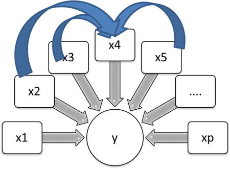
Figure 11-10. Multicollinearity in linear regression
You need to take the note of one fact here; multicollinearity is connected with independent variables, and their relation with the dependent variable has nothing to do with it. Whether it is a linear regression or a nonlinear regression, you can have scenarios where the independent variables are interdependent (Figure 11-11).

Figure 11-11. Multicollinearity in nonlinear regression
In simple terms, multicollinearity is an issue with logistic regression as well. The dependent variable is nowhere on the scene while you are dealing with multicollinearity. So, it doesn’t really matter whether you are building a linear or nonlinear regression model. Multicollinearity dents the accuracy of a logistic regression model as well. You have to be careful of multicollinearity while fitting a multiple logistic regression line. The steps are same as discussed in linear regression multicollinearity, shown here:
- Detect or conform multicollinearity using VIF values. If VIF is more than 5, then there is some multicollinearity within the independent variables.
- Once you find the existence of multicollinearity, you can drop one of the troublesome variable by looking at the individual variable’s Wald Chi-square value. Keep the variables that have a higher Wald Chi-square value.
No VIF Option in PROC LOGISTIC
Multicollinearity has nothing to do with logistic or linear regression. This phenomenon is entirely centered on independent variables. Accordingly, SAS doesn’t have a separate option of VIF in logistic regression. You have to follow the same steps as you followed with linear regression as far as the detection of multicollinearity is concerned. For variable selection or dropping, you can use logistic regression. In simple words, PROC LOGISTIC doesn’t have a VIF option; only PROC REG has that option.
If you write the VIF option in logistic regression, then SAS gives you an error. The following is one such example:
NOTE: The SAS System stopped processing this step because of errors.
704  proc logistic data=loans_data;
705  model SeriousDlqin2yrs = utilization Age Num_loans Num_dependents MonthlyIncome
705! Num_Savings_Acccts DebtRatio/vif;
                                  ---
                                  22
                                  202
ERROR 22-322: Syntax error, expecting one of the following: ;, ABSFCONV, AGGREGATE, ALPHA,
              BACKWARD, BEST, BINWIDTH, BUILDRULE, CL, CLODDS, CLPARM, CODING, CONVERGE,
              CORRB, COVB, CT, CTABLE, DETAILS, DSCALE, EXPB, FAST, FCONV, FIRTH, GCONV,
              HIERARCHY, INCLUDE, INFLUENCE, IPLOTS, ITPRINT, L, LACKFIT, LINK, MAXITER,
              MAXSTEP, NOCHECK, NODUMMYPRINT, NOFIT, NOINT, NOLOGSCALE, OFFSET, OUTROC,
              PARMLABEL, PEVENT, PL, PLCL, PLCONV, PLRL, PPROB, PSCALE, RIDGING, RISKLIMITS,
              ROCEPS, RSQUARE, SCALE, SELECTION, SEQUENTIAL, SINGULAR, SLE, SLENTRY, SLS,
              SLSTAY, START, STB, STEPWISE, STOP, STOPRES, TECHNIQUE, WALDCL, WALDRL, XCONV.
ERROR 202-322: The option or parameter is not recognized and will be ignored.
706  run;
So, in the case of logistic regression, you have to use PROC REG and follow the procedure explained in Chapter 10.
Logistic Regression Final Check List
Up to this point, we have discussed all the important concepts related to regression analysis. Logistic regression is just another type of regression. It is one of the most widely used nonlinear regression models across numerous industry verticals. The following is a check list to be used while building a logistic regression model:
- Applicability: Look at the data and the dependent variables. Is it categorical? Yes/No, 0/1, Win/Loss, and so on, are the types of response variable outcomes where you can apply logistic regression.
- Chi-square value: Look at the overall Chi-square value to decide whether a model is significant. If the Chi-square test fails, then stop it right there; the overall model itself is not significant. Chi-square is not going to tell you anything about the precise accuracy of a model.
- VIF: The multicollinearity issue needs to be solved in same fashion as in linear regression models (using PROC REG with the VIF option). Identify and resolve it by dropping the troublesome variables or by using PCA or FA, as explained in regression analysis in Chapter 10.
- Overall accuracy/concordance: Determine the accuracy of a mode by looking at its concordance and C values. The higher the value, the better the model. If the values of concordance and C are not satisfactory, then you may think of collecting some more data or adding better, more impactful independent variables, which will improve the overall model performance.
- Individual impact/Wald Chi-square value: Look at the individual impact of each variable by looking at the Wald Chi-square value. Drop the insignificant variables
Loan Default Prediction Case Study
As we have done throughout this book, we will revise the concepts learned in this chapter using a real-life case study.
Background and Problem Statement
ABC Bank has a personal loan product. It needs to be very sure about the payback capability of customers before it can approve a loan. The bank gets thousands of loan applications from its prospective customers, and it needs to have a flawless scientific method to approve or reject the loan applications. The bank decides to use data analytics to judge the risk associated with each customer.
ABC Bank has tons of historical data on customer profiles, their previous loans, their credit card spending, their bank accounts, and so on. The bank has historic data of both creditworthy and non-credit-worthy customers. Identifying the non-credit-worthy applicants before approving a loan saves millions of dollars for the bank. So, it is important to quantify the risk associated with each customer at the time of loan approval.
Analyze the historical loans data and build a model that will help the bank segregate the customers, based on the associated risk, at the time of loan approval.
Data Set
The bank’s historical data contains the records of both defaults and nondefaulters. It is collected over a period of two years. The data set has a record of 150,000 customers. It also has a response/dependent variable, which indicates the creditworthiness of each customer. Some predictor/independent variables are also there in each record, which indicate the customer’s financial health. The data set given here is reasonably clean for the model-building exercise. The data validation and sanitization have already been done. Also, there are no outliers or missing values in the variables.
Table 11-15 contains the details of the data set (the data dictionary).
Table 11-15. The Details of Data Set Used in the ABC Bank Example
|
Variable Name |
Description |
Type |
|---|---|---|
|
Cust_id |
Customer ID; unique for each customer. |
Number |
|
SeriousDlqin2yrs |
Person experienced BK/CO. BK: Bankruptcy. This is when a debtor realizes that she is unable to pay her bills. When any individual or business is unable to pay their creditors, bankruptcy is a legal option that can help them to get relief from their due payments and debt. CO: A customer fails to make the minimum payment due for a period of six months or more. 1 – Yes BK or CO: Bad customer. 0 – No BK or CO: Good customer. |
1/0 |
|
Utilization |
Average monthly utilization of credit limit. |
Percentage |
|
Age |
Age of the customer. |
Number |
|
Num_loans |
Number of loans including mortgage, vehicle, and personal loans. |
Number |
|
Num_dependents |
Number of dependents. | |
|
MonthlyIncome |
Average monthly income of the customer. |
Number |
|
Num_Savings_Acccts |
Number of savings accounts a customer has. |
Number |
|
DebtRatio |
Monthly debt payments, alimony, living costs divided by monthly gross income. |
Percentage |
Data Import
As a first step, you will import the data and do a quick check on the number of records, variables, formats, and so on.
The following is the code for importing the data set Customer_Loans.csv:
PROC IMPORT OUT= WORK.loans_data
            DATAFILE= "C:UsersVENKATGoogle DriveTrainingBooksContent11.
Logistic RegressionData Logistic RegressionCustomer_Loans.csv"
            DBMS=CSV REPLACE;
     GETNAMES=YES;
     DATAROW=2;
RUN;
Here are the notes from the log file for the previous code:
NOTE: The infile 'C:UsersVENKATGoogle DriveTrainingBooksContent11. Logistic
      RegressionData Logistic RegressionCustomer_Loans.csv' is:

      Filename=C:UsersVENKATGoogle DriveTrainingBooksContent11. Logistic
      RegressionData Logistic RegressionCustomer_Loans.csv,
      RECFM=V,LRECL=32767,File Size (bytes)=6918139,
      Last Modified=28Aug2014:11:52:33,
      Create Time=28Aug2014:11:12:22

NOTE: 150000 records were read from the infile 'C:UsersVENKATGoogle
      DriveTrainingBooksContent11. Logistic RegressionData Logistic
      RegressionCustomer_Loans.csv'.
      The minimum record length was 26.
      The maximum record length was 48.
NOTE: The data set WORK.LOANS_DATA has 150000 observations and 9 variables.
NOTE: DATA statement used (Total process time):
      real time           1.23 seconds
      cpu time            1.24 seconds

150000 rows created in WORK.LOANS_DATA from C:UsersVENKATGoogle
DriveTrainingBooksContent11. Logistic RegressionData Logistic
RegressionCustomer_Loans.csv.

NOTE: WORK.LOANS_DATA data set was successfully created.
NOTE: PROCEDURE IMPORT used (Total process time):
      real time           1.49 seconds
      cpu time            1.51 seconds
The following is the code for PROC CONTENTS and print data to see the variables and the snapshot of the data:
proc contents data=loans_data varnum;
run;

proc print data=loans_data(obs=20);
run;
Tables 11-16 and 11-17 list the output of these code snippets.
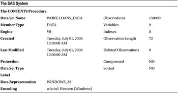
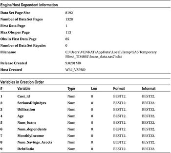

You have all the variables in the data, and it looks like all the variables are populated. The data looks clean. If not, you need to first explore the data, validate it for the accuracy, and finally clean it by treating missing values and outliers in the data. You need to use SAS procedures such as PROC CONTENTS, PROC FREQ, and PROC UNIVARIATE, which have been discussed at length in data exploration in Chapter 7.
The response variable in the data set is binary. SeriousDlqin2yrs is the dependent variable that you are planning to predict. It takes two values:
- 1, Yes BK or CO: Bad customer
- 0, No BK or CO: Good customer
Logistic regression is a good choice for predicting the default probability of a customer based on characteristics such as number of loans, debt ratio, monthly income, and so on.
The following is the code for building a logistic regression line:
proc logistic data=loans_data;
model SeriousDlqin2yrs = utilization Age Num_loans Num_dependents MonthlyIncome Num_Savings_Acccts DebtRatio;
run;
The following are the messages from the log file when the previous code was executed:
701  proc logistic data=loans_data;
702  model SeriousDlqin2yrs = utilization Age Num_loans Num_dependents MonthlyIncome
702! Num_Savings_Acccts DebtRatio;
703  run;

NOTE: Writing HTML Body file: sashtml44.htm
NOTE: PROC LOGISTIC is modeling the probability that SeriousDlqin2yrs='0'. One way to change
      this to model the probability that SeriousDlqin2yrs='1' is to specify the response
      variable option EVENT='1'.
NOTE: Convergence criterion (GCONV=1E-8) satisfied.
NOTE: There were 150000 observations read from the data set WORK.LOANS_DATA.
NOTE: PROCEDURE LOGISTIC used (Total process time):
      real time           4.92 seconds
      cpu time            3.58 seconds
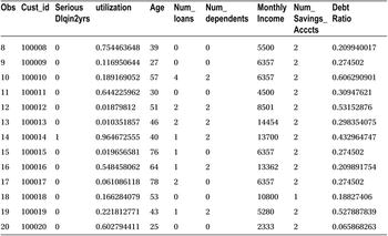
Table 11-18 shows the SAS output for this code.
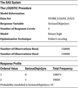
Now we will discuss the output in detail.
Some 150,000 customer records are read from the data set (Table 11-19) and are being used for this analysis. There are 139,974 good accounts and 10,026 bad accounts (Table 11-20). In the real-life bank loan portfolios, you would expect more than 90 percent of customers are good.
You may be wondering what you are trying to predict if good and bad accounts are already given. Why don’t you directly use them? Remember, this is historical data, where you already know who is good and who is bad. You are trying to use this data to fit a model, which will predict the probability of default (by new customers), given independent variables such as income, loans, debits, and utilization. You can use this model for future loan approvals for the new customers, even if they are not in the historic data. For all future customers, you will solicit the data on independent variables at the time of loan application, which will be used to assess the risk associated with each customer.
Of the following tables, Table 11-21 talks about the model convergence and Table 11-22 gives the Chi-square test results.
Table 11-19. Number of Observations in loans_data
|
Number of Observations Read |
150000 |
|---|---|
|
Number of Observations Used |
150000 |
Table 11-20. Frequency of 0 and 1 in SeriousDlqin2yr Variable
|
Response Profile | |||
|---|---|---|---|
|
Ordered Value |
SeriousDlqin2yrs |
Total Frequency | |
|
1 |
0 |
139974 | |
|
2 |
1 |
10026 | Probability modeled is SeriousDlqin2yrs=‘0 |
Table 11-21. Model Convergence Status
|
Model Convergence Status |
|---|
|
Convergence criterion (GCONV=1E-8) satisfied. |
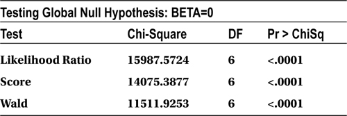
Looking at the Chi-square test results of the output (Table 11-22), you can confirm that the model is significant. All the P-values for the Chi-square tests are less than 5 percent (0.05). So, it is safe to conclude that the model is significant. In other words, at least one variable in the independent variables list has a significant impact on the response/dependent variable (SeriousDlqin2yrs). Take a look at the goodness of fit discussed earlier in the chapter to get a clear idea of how to interpret Table 11-22.
Table 11-22. Chi-square Test Results for the Model
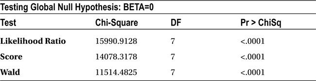
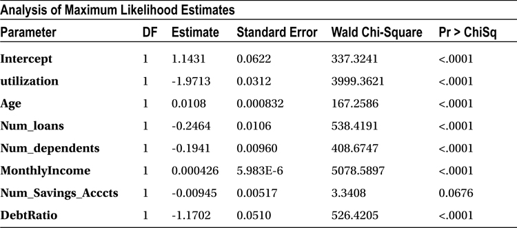
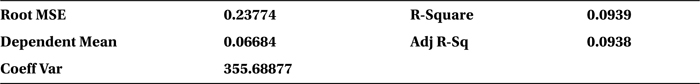
Table 11-23 is about variable coefficient estimates. The variable signs indicate that some of them have positive impact on dependent variable, while others impact negatively. Before looking at the sign of coefficients and their values or making any attempt to write the model equation, you need to make sure there is no interdependency within the independent variables. You are well aware that multicollinearity is a concern in logistic regression as well. You can’t trust these coefficients unless you make sure that there is no multicollinearity in the model.
Table 11-23. Variable Coefficient Estimates
To reiterate, multicollinearity is an issue affected by only the list of independent variables. It has nothing to do with the relation of the independent variables to the dependent variables. Whether you are building a linear or logistic regression line, the treatment of the multicollinearity issue remains the same.
The following is the code for detecting multicollinearity using the VIF option:
proc logistic data=loans_data;
model SeriousDlqin2yrs = utilization Age Num_loans Num_dependents MonthlyIncome Num_Savings_Acccts DebtRatio/vif;
run;
Remember that PROC LOGISTIC has no VIF option. If a VIF option is used, this PROC code throws an error, as shown here:
NOTE: The SAS System stopped processing this step because of errors.
704  proc logistic data=loans_data;
705  model SeriousDlqin2yrs = utilization Age Num_loans Num_dependents MonthlyIncome
705! Num_Savings_Acccts DebtRatio/vif;
                                  ---
                                  22
                                  202
ERROR 22-322: Syntax error, expecting one of the following: ;, ABSFCONV, AGGREGATE, ALPHA,
              BACKWARD, BEST, BINWIDTH, BUILDRULE, CL, CLODDS, CLPARM, CODING, CONVERGE,
              CORRB, COVB, CT, CTABLE, DETAILS, DSCALE, EXPB, FAST, FCONV, FIRTH, GCONV,
              HIERARCHY, INCLUDE, INFLUENCE, IPLOTS, ITPRINT, L, LACKFIT, LINK, MAXITER,
              MAXSTEP, NOCHECK, NODUMMYPRINT, NOFIT, NOINT, NOLOGSCALE, OFFSET, OUTROC,
              PARMLABEL, PEVENT, PL, PLCL, PLCONV, PLRL, PPROB, PSCALE, RIDGING, RISKLIMITS,
              ROCEPS, RSQUARE, SCALE, SELECTION, SEQUENTIAL, SINGULAR, SLE, SLENTRY, SLS,
              SLSTAY, START, STB, STEPWISE, STOP, STOPRES, TECHNIQUE, WALDCL, WALDRL, XCONV.
ERROR 202-322: The option or parameter is not recognized and will be ignored.
706  run;
So, you need to use PROC REG for the treatment of multicollinearity here as well.
proc reg data=loans_data;
model SeriousDlqin2yrs = utilization Age Num_loans Num_dependents MonthlyIncome Num_Savings_Acccts DebtRatio/vif;
run;
Table 11-24 shows the output for the previous code.
Table 11-24. Output of proc reg on loans_data
|
The SAS System | |
|---|---|
|
The REG Procedure | |
|
Model: MODEL1 | |
|
Dependent Variable: SeriousDlqin2yrs | |
|
Number of Observations Read |
150000 |
|
Number of Observations Used |
150000 |
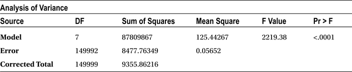
In this case, you don’t really care about R-square or the adjusted R-square. The only table that you are going to focus on in this output is the Parameter Estimates table. In particular, you are interested only in VIF values, which give you an indication about the multicollinearity. None of the variables has a VIF value of more than 5, which indicates that there is no interdependency in the independent variables. So, you can keep all the independent variables while building the logistic regression model.
Predicting Delinquency
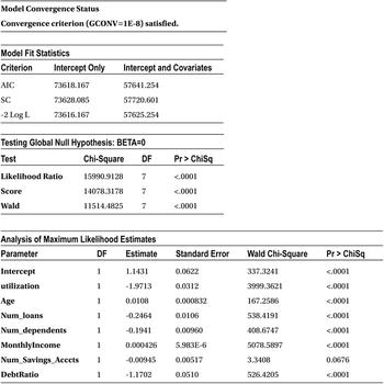
You can see a note in the output saying “Probability modeled is SeriousDlqin2yrs=‘0’,” which means the resultant probability from the model will be the probability of good. This would mean the higher the probability, the better the customer. If you want to predict the probability of bad instead of the probability of good, you have to use the descending option in the PROC LOGISTIC code. Most of the time, you try to predict the probability of the default rather than the probability of the nondefault. The following is the code for the final model. Remember, this will change the coefficients as well.
proc logistic data=loans_data descending;
model SeriousDlqin2yrs = utilization Age Num_loans Num_dependents MonthlyIncome Num_Savings_Acccts DebtRatio;
run;
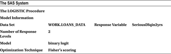
Table 11-25 shows the output of this code.
Table 11-25. Output of proc logistic on loans_data
|
The SAS System | |
|---|---|
|
The LOGISTIC Procedure | |
|
Model Information | |
|
Data Set |
WORK.LOANS_DATA |
|
Response Variable |
SeriousDlqin2yrs |
|
Number of Response Levels |
2 |
|
Model |
binary logit |
|
Optimization Technique |
Fisher’s scoring |
|
Number of Observations Read |
150000 |
|
Number of Observations Used |
150000 |
|
Response Profile | ||
|---|---|---|
|
Ordered Value |
SeriousDlqin2yrs |
Total Frequency |
|
1 |
0 |
139974 |
2 |
1 |
10026 |
| Probabilitymodeled is SeriousDlqin2yrs=‘1’. | ||
|
Model Convergence Status |
|
Convergence criterion (GCONV=1E-8) satisfied. |
|
Model Fit Statistics | ||
|---|---|---|
|
Criterion |
Intercept Only |
Intercept and Covariates |
|
AIC |
73618.167 |
57641.254 |
|
SC |
73628.085 |
57720.601 |
|
-2 Log L |
73616.167 |
57625.254 |

Now you can observe that the note has changed in the SAS output. If a customer scores high in this model, then she has a higher probability to default in the repayment of the loan. The following is the note, reproduced from the SAS output in Table 11-25.
Probability modeled is SeriousDlqin2yrs=‘1’.
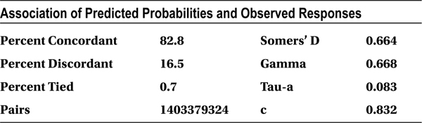
Goodness of Fit Statistic
The concordance is 82.8 percent, and the discordance is 16.5 percent, which is really good for any logistic regression model. In real-life business problems, generally it is desirable to have a concordance of 75 percent or more. You can go ahead and use this model for prediction with greater confidence.
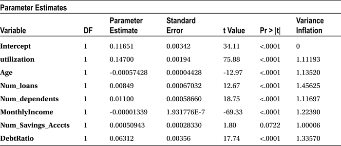
Insignificant Variables
Before you use this model for predictions, you have to see whether there are any independent variables that have no significant impact on the dependent variable. You can take a look at the P-value of individual independent variables (Table 11-26) to get an idea on their importance in the model. Any variable with a P-value of more than 5 percent in the Chi-square test is insignificant in the model. The predictions using this model will not be affected at all by keeping or removing such variables.
Table 11-26. Variable Coefficient Estimates
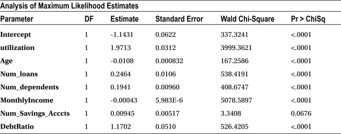
In this data set, the number of savings accounts has no significant impact on the delinquency of a customer (P-value = 0.0676). Table 11-27 shows the goodness of fit statistics keeping the number of savings account variable in the model.
Table 11-27. Goodness of Fit Statistics
|
Percent Concordant |
82.8 |
|---|---|
|
Percent Discordant |
16.5 |
Let’s see how the accuracy will change if you drop this variable from the final model. Ideally there should be no effect on the accuracy of the model because the variable is insignificant.
/* Final Model after Dropping Num_Savings_Acccts */
proc logistic data=loans_data descending;
model SeriousDlqin2yrs = utilization Age Num_loans Num_dependents MonthlyIncome DebtRatio;
run;
The following is the output, which indicates there is absolutely no change in accuracy even after dropping the number of savings accounts variable.
|
Percent Concordant |
82.8 |
|
Percent Discordant |
16.5 |
Final Model
The following is the code for creating the final logistic regression model:
proc logistic data=loans_data descending;
model SeriousDlqin2yrs = utilization Age Num_loans Num_dependents MonthlyIncome DebtRatio;
run;
Table 11-28 is the output for the previous code.
Table 11-28. Output of proc logistic after Dropping Num_Savings_Acccts
|
Number of Observations Read |
150000 |
|
Number of Observations Used |
150000 |
|
Response Profile | ||
|
Ordered Value |
SeriousDlqin2yrs |
Total Frequency |
|---|---|---|
|
1 |
1 |
10026 |
|
2 |
0 |
139974 |
| Probability modeled is SeriousDlqin2yrs=‘1’. | ||
|
Model Convergence Status |
|
Convergence criterion (GCONV=1E-8) satisfied. |
|
Model Fit Statistics | ||
|
Criterion |
Intercept Only |
Intercept and Covariates |
|---|---|---|
|
AIC |
73618.167 |
57642.594 |
|
SC |
73628.085 |
57712.023 |
|
-2 Log L |
73616.167 |
57628.594 |


The following is the final check list:
- Applicability: A linear regression model can’t be applied for this data because the response variable is categorical (0 and 1). Logistic regression is a perfect fit for this dependent variable, which is binary in nature.
- Chi-square test: The P-value of the overall model Chi-square test is less than 5 percent, so the model can be termed significant.
- VIF: None of the variables has a VIF of more than 5 percent, so there is absolutely no multicollinearity.
- Concordance: The model concordance is 82.8 percent, which indicates that the resultant model is going to be a good predictor.
- Individual variable impact: The P-values for all the independent variables (finally included in the model) are less than 5 percent, which indicates there are no insignificant variables in the final model. One insignificant variable was already dropped.
Final Model Equation and Prediction Using the Model
Here is the final model after substituting all the coefficients:

Predictions Using the Model
The bank can use the final model for quantifying the risk associated with each customer at the time of loan approval. The model gives the probability of default, so the bank can set a minimum limit, which may be that if any customer has a probability of default greater than 50 percent, as given by this model, the application will be rejected.
For example, consider the three customers shown in Table 11-29 with the details furnished in their loan applications.
Table 11-29. Details in the Loan Application for Example Customers

You can get the calculated probability values (Table 11-30) by substituting these values in the logistic regression equation:

Table 11-30. The Predicted Default Probabilities
|
Customer |
Predicted Default Probability |
Decision |
|---|---|---|
|
Tom |
0.0047 (5%) |
Approve the loan |
|
David |
0.56 (56%) |
Reject the loan application |
|
Hanks |
0.79 (79%) |
Reject the loan application |
So, only Tom gets a loan. Generally, banks might not reject all the customers with a greater than 50 percent probability. They might approve lesser value loans for the risky customers or charge higher interest rates and reduce the loan amount. Table 11-31 might be an example of a moderated implementation of the final defaulter model.
Table 11-31. Decision Making Using the Default Probability Range
|
Default Probability Range |
Decision |
|---|---|
|
0%-45% |
Approve loan application |
|
45%-65% |
Approve loan application with reduced loan amount |
|
65% |
Decline the loan application |
Banks will send this model and the decision table to their front-end teams or install the model in a centralized system, which can be accessed by its loans processing team. It will be used as a primary tool for assessing any loan application. The decision methodology is scientific and reasonably accurate and uses analytics on the associated customer data.
Conclusion
In this chapter, we discussed that linear regression is not applicable for binary dependent variables. A logistic curve is best suited for such dependent variables. If the dependent variable has only two levels, you need to use logistic regression, which is also known as binomial logistic regression. If the response variable has more than two levels, such as good/bad/indeterminate, win/loss/draw, or satisfied/dissatisfied/neutral, then you need to use multinomial logistic regression.
You learned how to fit a logistic regression line using SAS and also observed some of the similarities and differences in the output (with linear regression). The logistic regression line also suffers from multicollinearity issues; however, the process of treating multicollinearity is the same as in linear regression. There are other nonlinear regressions as well. Logistics is not the only nonlinear regression. You have finished the regression-related topics with this chapter and will get into other methods of modeling such as ARIMA in the following chapters.