
Chapter 14. Building the Purrfect Cat Locator App with TensorFlow Object Detection API
Bob gets frequent visits from a neighborhood feral cat. Those visits result in less than pleasant outcomes. You see, Bob has a nice fairly large garden that he tends to with great care. However, this furry little fella visits his garden every night and starts chewing on a bunch of plants. Months of hard work gets destroyed overnight. Clearly unhappy with this situation, Bob is keen on doing something about it.
Channeling his inner Ace Ventura (Pet Detective), he tries to stay awake at night to drive the cat away, but clearly, that’s not sustainable in the long term. After all, Red Bull has its limits. Reaching a breaking point, he decides to use the nuclear option: use AI in conjunction with his sprinkler system to literally “turn the hose” on the cat.
In his sprawling garden, he sets up a camera that can track the motion of the cat and turn on the nearest set of sprinklers to scare the cat away. He has an old phone lying around, and all he needs is a way to determine the cat’s location in real time, so he can control accordingly which sprinkler to trigger.
Hopefully, after a few unwelcome baths, as demonstrated in Figure 14-1, the cat would be disincentivized from raiding Bob’s garden.

Figure 14-1. Building an AI cat sprinkler system, like this Havahart Spray Away Motion Detector
Tip
Keen observers might have noticed that we’re attempting to find the position of the cat in 2D space, whereas the cat itself exists in 3D space. We can make assumptions to simplify the problem of locating the cat in real-world coordinates by assuming that the camera will always be in a fixed position. To determine the distance of the cat, we can use the size of an average cat to take measurements of its apparent size on a picture at regular intervals of distance from the camera. For example, an average cat might appear to have a bounding box height of 300 pixels at a distance of two feet from the camera, whereas it might occupy 250 pixels when it’s three feet away from the camera lens.
In this chapter, we help Bob make his cat detector. (Note to animal-rights advocates: no cats were harmed in the making of this chapter.) We answer the following questions along the way:
-
What are the different kinds of computer-vision tasks?
-
How do I reuse a model pretrained for an existing class of objects?
-
Can I train an object detector model without writing any code?
-
I want more granular control for greater accuracy and speed. How do I train a custom object detector?
Types of Computer-Vision Tasks
In most of the previous chapters, we’ve essentially looked at one kind of problem: object classification. In that, we found out whether an image contained objects of a certain class. In Bob’s scenario, in addition to knowing whether the camera is seeing a cat, it is necessary to know exactly where the cat is in order to trigger the nearest sprinkler. Determining the location of an object within an image is a different type of problem: object detection. Before we jump into object detection, let’s look at the variety of frequent computer-vision tasks and the questions they purport to answer.
Classification
We have looked at several examples of classification throughout this book. Simply put, the task of classification assigns an image with the class(es) of the object(s) present in the image. It answers the question: “Is there an object of class X in the image?” Classification is one of the most fundamental computer-vision tasks. In an image, there might be objects of more than one class—called multiclass classification. The label in this case for one image would be a list of all object classes that the image contains.
Localization
The downside of classification is that it does not tell us where in the image a particular object is, how big or small it is, or how many objects there are. It only tells us that an object of a particular class exists somewhere within it. Localization, otherwise known as classification with localization, can inform us which classes are in an image and where they are located within the image. The keyword here is classes, as opposed to individual objects, because localization gives us only one bounding box per class. Just like classification, it cannot answer the question “How many objects of class X are in this image?”
As you will see momentarily, localization will work correctly only when it is guaranteed that there is a single instance of each class. If there is more than one instance of a class, one bounding box might encompass some or all objects of that class (depending upon the probabilities). But just one bounding box per class seems rather restrictive, doesn’t it?
Detection
When we have multiple objects belonging to multiple classes in the same image, localization will not suffice. Object detection would give us a bounding rectangle for every instance of a class, for all classes. It also informs us as to the class of the object within each of the detected bounding boxes. For example, in the case of a self-driving car, object detection would return one bounding box per car, person, lamp post, and so on that the car sees. Because of this ability, we also can use it in applications that need to count. For example, counting the number of people in a crowd.
Unlike localization, detection does not have a restriction on the number of instances of a class in an image. This is why it is used in real-world applications.
Segmentation
Object segmentation is the task of assigning a class label to individual pixels throughout an image. A children’s coloring book where we use crayons to color various objects is a real-world analogy. Considering each pixel in the image is being assigned a class, it is a highly compute-intensive task. Although object localization and detection give bounding boxes, segmentation produces groups of pixels—also known as masks. Segmentation is obviously much more precise about the boundaries of an object compared to detection. For example, a cosmetic app that changes a user’s hair color in real-time would use segmentation. Based on the types of masks, segmentation comes in different flavors.
Semantic segmentation
Given an image, semantic segmentation assigns one mask per class. If there are multiple objects of the same class, all of them are assigned to the same mask. There is no differentiation between the instances of the same class. Just like localization, semantic segmentation cannot count.
Instance-level segmentation
Given an image, instance-level segmentation identifies the area occupied by each instance of each class. Different instances of the same class will be segmented uniquely.
Table 14-1 lists the different computer-vision tasks.
| Task | Image | In lay terms | Outputs |
|---|---|---|---|
| Object classification |
 |
Is there a sheep in this image? | Class probabilities |
| Object localization |
 |
Is there “a” sheep in the image and where is it? | Bounding box and class probability |
|
Object detection |
 |
What and where are “all” the objects in this image? | Bounding boxes, class probabilities, class ID prediction |
| Semantic segmentation |
 |
Which pixels in this image belong to different classes; e.g., the class “sheep,” “dog,” “person”? | One mask per class |
| Instance-level segmentation |
 |
Which pixels in this image belong to each instance of each class; e.g., “sheep,” “dog,” “person”? | One mask per instance of each class |
Approaches to Object Detection
Depending on the scenario, your needs, and technical know-how, there are a few ways to go about getting the object detection functionality in your applications. Table 14-2 takes a look at some approaches.
| Custom classes | Effort | Cloud or local | Pros and cons | |
|---|---|---|---|---|
| Cloud-based object detection APIs | No | <5 minutes | Cloud only |
+ Thousands of classes + State of the art + Fast setup + Scalable API – No customization – Latency due to network |
| Pretrained model | No | <15 minutes | Local |
+ ~100 classes + Choice of model to fit speed and accuracy needs + Can run on the edge – No customization |
| Cloud-based model training | Yes | <20 minutes | Cloud and local |
+ GUI-based, no coding for training + Customizability + Choice between powerful model (for cloud) and efficient model (for edge) + Scalable API – Uses transfer learning, might not allow full-model retraining |
| Custom training a model | Yes | 4 hours to 2 days | Local |
+ Highly customizable + Largest variety of models available for different speed and accuracy requirements – Time consuming and highly involved |
It’s worth noting that the options marked “Cloud” are already engineered for scalability. At the same time, the options marked as being available for “Local” inferences can also be deployed on the cloud. To achieve high scale, we can host them on the cloud similar to how we did so for the classification models in Chapter 9.
Invoking Prebuilt Cloud-Based Object Detection APIs
As we already saw in Chapter 8, calling cloud-based APIs is relatively straightforward. The process involves setting up an account, getting an API key, reading through the documentation, and writing a REST API client. To make this process easier, many of these services provide Python-based (and other language) SDKs. The main cloud-based object detection API providers are Google’s Vision AI (Figure 14-2) and Microsoft’s Cognitive Services.
The main advantages of using cloud-based APIs are that they are scalable out of the box and they support recognition of thousands of classes of objects. These cloud giants built their models using large proprietary datasets that are constantly growing, resulting in a very rich taxonomy. Considering that the number of classes in the largest public datasets with object detection labels is usually only a few hundred, there exists no nonproprietary solution out there that is capable of detecting thousands of classes.
The main limitation of cloud-based APIs, of course, is the latency due to network requests. It’s not possible to power real-time experiences with this kind of lag. In the next section, we look at how to power real-time experiences without any data or training.

Figure 14-2. Running a familiar photo on Google’s Vision AI API to obtain object detection results
Reusing a Pretrained Model
In this section, we explore how easy it is to get an object detector running on a mobile phone with a pretrained model. Hopefully, you are already comfortable with running a neural network on mobile from some of the previous chapters. The code to run object detection models on iOS and Android is referenced on the book’s GitHub website (see http://PracticalDeepLearning.ai) at code/chapter-14. Changing functionality is simply a matter of replacing the existing .tflite model file with a new one.
In the previous chapters, we often used MobileNet to do classification tasks. Although the MobileNet family, including MobileNetV2 (2018) and MobileNetV3 (2019) by itself are classification networks only, they can act as a backbone for object detection architectures like SSD MobileNetV2, which we use in this chapter.
Obtaining the Model
The best way to uncover the magic behind the scenes is to take a deeper look at a model. We’d need to get our hands on the TensorFlow Models repository, which features models for more than 50 deep learning tasks, including audio classification, text summarization, and object detection. This repository contains models as well as utility scripts that we use throughout this chapter. Without further ado, let’s clone the repository on our machines:
$ git clone https://github.com/tensorflow/models.git && cd models/research
Then, we update the PYTHONPATH to make all scripts visible to Python:
$ export PYTHONPATH="${PYTHONPATH}:`pwd`:`pwd`/slim"
Next, we copy over the Protocol Buffer (protobuf) compiler command script from our GitHub repository (see http://PracticalDeepLearning.ai) into our current directory to make the .proto files available to Python:
$ cp {path_to_book_github_repo}/code/chapter-14/add_protoc.sh . &&
chmod +x add_protoc.sh &&
./add_protoc.sh
Finally, we run the setup.py script as follows:
$ python setup.py build
$ python setup.py install
Now is the time to download our prebuilt model. In our case, we’re using the SSD MobileNetV2 model. You can find a large list of models at TensorFlow’s object detection model zoo, featuring models by the datasets on which they were trained, speed of inference, and Mean Average Precision (mAP). Within that list, download the model titled ssd_mobilenet_v2_coco, which, as the name suggests, was trained on the MS COCO dataset. Benchmarked at 22 mAP, this model runs at 31 ms on an NVIDIA GeForce GTX TITAN X with a 600x600 resolution input. After downloading that model, we unzip it into the models/research/object_detection directory inside the TensorFlow repository. We can inspect the contents of the directory as follows:
$ cd object_detection/
$ ls ssd_mobilenet_v2_coco_2018_03_29
checkpoint                      model.ckpt.data-00000-of-00001  model.ckpt.meta
saved_model
frozen_inference_graph.pb       model.ckpt.index                pipeline.config
Test Driving Our Model
Before we plug our model into a mobile app, it’s a good idea to verify whether the model is able to make predictions. The TensorFlow Models repository contains a Jupyter Notebook where we can simply plug in a photograph to make predictions on it. You can find the notebook at models/research/object_detection/object_detection_tutorial.ipynb. Figure 14-3 shows a prediction from that notebook on a familiar photograph.

Figure 14-3. Object detection prediction in the ready-to-use Jupyter Notebook from the TensorFlow Models repository
Deploying to a Device
Now that we’ve verified that the model works, it’s time to convert it into a mobile-friendly format. For conversion to the TensorFlow Lite format, we use our familiar tflite_convert tool from Chapter 13. It should be noted that this tool operates on .pb files, whereas the TensorFlow Object Detection model zoo provides only model checkpoints. So, we first need to generate a .pb model from the checkpoints and graphs. Let’s do that using the handy script that comes with the TensorFlow Models repository. You can find the export_tflite_ssd_graph.py file in models/research/object_detection:
$ python export_tflite_ssd_graph.py
--pipeline_config_path=ssd_mobilenet_v2_coco_2018_03_29/pipeline.config
--trained_checkpoint_prefix=ssd_mobilenet_v2_coco_2018_03_29/
model.ckpt.data-00000-of-00001
--output_directory=tflite_model
--add_postprocessing_op=true
If the preceding script execution was successful, we’ll see the following files in the tflite_model directory:
$ ls tflite_model
tflite_graph.pb
tflite_graph.pbtxt
We will convert this to the TensorFlow Lite format using the tflite_convert tool.
$ tflite_convert --graph_def_file=tflite_model/tflite_graph.pb
--output_file=tflite_model/model.tflite
Now the only thing that remains is to plug the model into an app. The app that we’ll be using is referenced in the book’s GitHub website (see http://PracticalDeepLearning.ai) at code/chapter-14. We have already looked at how to swap a model in an app in Chapters 11, 12, and 13, so we won’t discuss that here again. Figure 14-4 shows the result of the object detector model when plugged into the Android app.

Figure 14-4. Running a real-time object detector model on an Android device
The reason why we’re able to see the “Cat” prediction right away is because ‘Cat’ is one of the 80 categories already present in the MS COCO dataset that was used to train the model. This model might be sufficient for Bob to deploy on his devices (keeping in mind that although Bob might not use mobile phones to track his garden, the process for deploying a TensorFlow Lite model to edge hardware is quite similar). However, Bob would do well for himself to improve the precision of his model by fine tuning it on data that has been generated within his garden. In the next section, we explore how to use transfer learning to build an object detector by using only a web-based tool. If you’ve read Chapter 8, what comes next should feel familiar.
Building a Custom Detector Without Any Code
My cat’s breath smells like cat food!
Ralph Wiggum
Let’s face it. Your authors could go around and snap a lot of cat pictures within their gardens to perform this experiment. It would be tedious, and we might be rewarded with only a few extra percentage points of precision and recall. Or we could look at a really fun example that also tests the limits of CNNs. We are, of course, referring to The Simpsons. Given that most models are not trained with features from cartoon images, it would be interesting to see how our model performs here.
First, we need to get our hands on a dataset. Thankfully, we have one readily available on Kaggle. Let’s download the dataset and use CustomVision.ai (similar to Chapter 8) to train our Simpsons Classifier using the following steps. Excellent!
Note
Contrary to what some may believe, we, the authors, do not have millions of dollars lying around. This means that we cannot afford to buy the rights to The Simpsons from Fox. Copyright laws, as a consequence, prevent us from publishing any images from that show. Instead, in this section, we are using the next best thing—public domain images from the United States Congress. In place of the images from the cartoon, we use the photographs of congresswomen and congressmen with the same first names as the Simpsons family: Homer Hoch, Marge Roukema, Bart Gordon, and Lisa Blunt Rochester. Keep in mind that this is only for publishing purposes; we have still trained on the original dataset from the cartoon.
-
Go to CustomVision.ai and start a new Object Detection Project (Figure 14-5).

Figure 14-5. Creating a new Object Detection project in CustomVision.ai
-
Create tags for Homer, Marge, Bart, and Lisa. Upload 15 images for each character and draw a bounding box for each of those images. The dashboard should resemble Figure 14-6 right about now.

Figure 14-6. Dashboard with bounding box and class name
-
Click the Train button and let the training commence. There are sliders to control the probability and overlap thresholds on the dashboard. We can play around with them and adjust them to something we like and with which get good precision and recall.
-
Click the Quick Test button and use any random image of the Simpsons (not previously used for training) to test the performance of the model. The results might not be great yet, but that’s okay: we can fix it by training with more data.
-
Let’s experiment with how many images we need to increase precision, recall, and mAP. Let’s start by adding five more images for each class and retrain the model.
-
Repeat this process until we have acceptable results. Figure 14-7 shows the results from our experiment.

Figure 14-7. Measuring improvement in percent mean average precision with increasing number of images per class
With our final model, we are able to get reasonably good detections for a random image off the internet, as can be seen in Figure 14-8. Although not expected, it is surprising that a model pretrained on natural images is able to fine tune on cartoons with relatively little data.

Figure 14-8. Detected Simpsons characters with the final model, represented by US congress members of the same first name (see note at the beginning of this section)
As we already know by now, CustomVision.ai allows this model to be exported in a variety of formats including Core ML, TensorFlow Lite, ONNX, and more. We can simply download into our desired format (.tflite in our case) and plug this file into the app similar to see how we did with the pretrained model in the previous section. With real-time Simpsons detection in our hands, we could show it off to our friends and family the next time Principal Skinner talks about steamed hams on our TV.
Note
CustomVision.ai is not the only platform that allows you to label, train, and deploy online without writing any code. Google’s Cloud AutoML (in beta as of October 2019) and Apple’s Create ML (only for the Apple ecosystem) offer a very similar feature set. Additionally, Matroid allows you to build custom object detectors from video feeds, which can be extremely useful to train a network without spending too much effort on building a dataset.
So far, we have looked at three quick ways to get object detection running with a very minimal amount of code. We estimate that about 90% of use cases can be handled with one of these options. If you can solve for your scenario using these, you can stop reading this chapter and jump straight to the “Case Studies” section.
In a very small set of scenarios, we might want further fine-grained control on factors such as accuracy, speech, model size, and resource usage. In the upcoming sections, we look at the world of object detection in a little more detail, from labeling the data all the way to deploying the model.
The Evolution of Object Detection
Over the years, as the deep learning revolution happened, there was a renaissance not only for classification, but also for other computer-vision tasks, including object detection. During this time, several architectures were proposed for object detection, often building on top of each other. Figure 14-9 shows a timeline of some of them.

Figure 14-9. A timeline of different object detection architectures (image source: Recent Advances in Deep Learning for Object Detection by Xiongwei Wu et al.)
In object classification, our CNN architecture extracts the features from an image and computes the probabilities for a specific number of classes. These CNN architectures (ResNet, MobileNet) work as the backbone for object detection networks. In object detection networks, our end result is bounding boxes (defined by the center of rectangle, height, width). Although covering the inner details of many of these will probably need significantly more in-depth exploration (which you can find on this book’s GitHub website, linked at http://PracticalDeepLearning.ai), we can broadly divide them into two categories, as shown in Table 14-3.
| Description | Pros and cons | |
|---|---|---|
| Two-stage detectors |
Generate category-agnostic bounding box candidates (regions of interest) using a Region Proposal Network (RPN). Run a CNN on these region proposals to assign each a category. Examples: Faster R-CNN, Mask R-CNN. |
+ High Accuracy – Slower |
| One-stage detectors |
Directly make categorical predictions on objects on each location of the feature maps; can be trained end-to-end training. Examples: YOLO, Single-Shot Detector (SSD). |
+ Speed, better suited for real-time applications – Lower accuracy |
Note
In the world of object detection, Ross Girshik is a name you will encounter often while reading papers. Working before the deep learning era as well as during it, his work includes Deformable Part Models (DPM), R-CNN, Fast R-CNN, Faster R-CNN, You Only Look Once (YOLO), Mask R-CNN, Feature Pyramid Network (FPN), RetinaNet, and ResNeXt to name just a few, often breaking his own records year after year on public benchmarks.
I participated in several first-place entries into the PASCAL VOC object detection challenge, and was awarded a “lifetime achievement” prize for my work on deformable part models. I think this refers to the lifetime of the PASCAL challenge—and not mine!
—Ross Girschik
Performance Considerations
From a practitioner’s point of view, the primary concerns tend to be accuracy and speed. These two factors usually have an inverse relationship with each other. We want to find the detector that strikes the ideal balance for our scenario. Table 14-4 summarizes some of those readily available pretrained models on the TensorFlow object detection model zoo. The speed reported was on a 600x600 pixel resolution image input, processed on an NVIDIA GeForce GTX TITAN X card.
| Inference speed (ms) | % mAP on MS COCO | |
|---|---|---|
| ssd_mobilenet_v1_coco | 30 | 21 |
| ssd_mobilenet_v2_coco | 31 | 22 |
| ssdlite_mobilenet_v2_coco | 27 | 22 |
| ssd_resnet_50_fpn_coco | 76 | 35 |
| faster_rcnn_nas | 1,833 | 43 |
A 2017 study done by Google (see Figure 14-10) revealed the following key findings:
-
One-stage detectors are faster than two-stage, though less accurate.
-
The higher the accuracy of the backbone CNN architecture on classification tasks (such as ImageNet), the higher the precision of the object detector.
-
Small-sized objects are challenging for object detectors, which give poor performance (usually under 10% mAP). The effect is more severe on one-stage detectors.
-
On large-sized objects, most detectors give similar performance.
-
Higher-resolution images give better results because small objects appear larger to the network.
-
Two-stage object detectors internally generate a large number of proposals to be considered as the potential locations of objects. The number of proposals can be tuned. Decreasing the number of proposals can lead to speedups with little loss in accuracy (the threshold will depend on the use case).

Figure 14-10. The effect of object detection architecture as well as the backbone architecture (feature extractor) on the percent mean average precision and prediction time (note that the colors might not be clear in grayscale printing; refer to the book’s GitHub website [see http://PracticalDeepLearning.ai] for the color image) (image source: Speed/accuracy trade-offs for modern convolutional object detectors by Jonathan Huang et al.)
Key Terms in Object Detection
The terms used heavily in object detection include Intersection over Union, Mean Average Precision, Non-Maximum Suppression, and Anchor. Let’s examine what each of these means.
Intersection over Union
In an object detection training pipeline, metrics such as Intersection over Union (IoU) are typically used as a threshold value to filter detections of a certain quality. To calculate the IoU, we use both the predicted bounding box and the ground truth bounding box to calculate two different numbers. The first is the area where both the prediction and the ground truth overlap—the intersection. The second is the span covered by both the prediction and the ground truth—the union. As the name suggests, we simply divide the total area of the intersection by the area of the union to get the IoU. Figure 14-11 visually demonstrates the IoU concept for two 2x2 squares that intersect in a single 1x1 square in the middle.

Figure 14-11. A visual representation of the IoU ratio
In the perfect scenario in which the predicted bounding box matches the ground truth exactly, the IoU value would be 1. In the worst-case scenario, the prediction would have no overlap with the ground truth and the IoU value would be 0. As we can see, the IoU value would range between 0 and 1, with higher numbers indicating higher-quality predictions, as illustrated in Figure 14-12.
To help us filter and report results, we would set a minimum IoU threshold value. Setting the threshold to a really aggressive value (such as 0.9) would result in a loss of a lot of predictions that might turn out to be important further down the pipeline. Conversely, setting the threshold value too low would result in too many spurious bounding boxes. A minimum IoU of 0.5 is typically used for reporting the precision of an object detection model.

Figure 14-12. IoU illustrated; predictions from better models tend to have heavier overlap with the ground truth, resulting in a higher IoU
It’s worth reiterating here that the IoU value is calculated per instance of a category, not per image. However, to calculate the quality of the detector over a larger set of images, we would use IoU in conjunction with other metrics such as Average Precision.
Mean Average Precision
While reading research papers on object detection, we often come across numbers such as [email protected]. That term conveys the average precision at IoU=0.5. Another more elaborate representation would be AP@[0.6:0.05:0.75], which is the average precision from IoU=0.6 to IoU=0.75 at increments of 0.05. The Mean Average Precision (or mAP) is simply the average precision across all categories. For the COCO challenge, the MAP metric used is AP@[0.5:0.05:0.95].
Non-Maximum Suppression
Internally, object detection algorithms make a number of proposals for the potential locations of objects that might be in the image. For each object in the image, it is expected to have multiple of these bounding box proposals at varying confidence values. Our task is to find the one proposal that best represents the real location of the object. A naïve way would be to consider only the proposal with the maximum confidence value. This approach might work if there were only one object in the entire image. But this won’t work if there are multiple categories, each with multiple instances in a single image.
Non-Maximum Suppression (NMS) comes to the rescue (Figure 14-13). The key idea behind NMS is that two instances of the same object will not have heavily overlapping bounding boxes; for instance, the IoU of their bounding boxes will be less than a certain IoU threshold (say 0.5). A greedy way to achieve this is by repeating the following steps for each category:
-
Filter out all proposals under a minimum confidence threshold.
-
Accept the proposal with the maximum confidence value.
-
For all remaining proposals sorted in descending order of their confidence values, check whether the IoU of the current box with respect to one of the previously accepted proposals ≥ 0.5. If so, filter it; otherwise, accept it as a proposal.

Figure 14-13. Using NMS to find the bounding box that best represents the location of the object in an image
Using the TensorFlow Object Detection API to Build Custom Models
In this section, we run through a full end-to-end example of building an object detector. We look at several steps in the process, including collecting, labeling, and preprocessing data, training the model, and exporting it to the TensorFlow Lite format.
First, let’s look at some strategies for collecting data.
Data Collection
We know by now that, in the world of deep learning, data reigns supreme. There are a few ways in which we can acquire data for the object that we want to detect:
- Using ready-to-use datasets
-
There are a few public datasets available to train object detection models such as MS COCO (80 categories), ImageNet (200 categories), Pascal VOC (20 categories), and the newer Open Images (600 categories). MS COCO and Pascal VOC are used in most object detection benchmarks, with COCO-based benchmarks being more realistic for real-world scenarios due to more complex imagery.
- Downloading from the web
-
We should already be familiar with this process from Chapter 12 in which we collected images for the “Hot Dog” and “Not Hot Dog” classes. Browser extensions such as Fatkun come in handy for quickly downloading a large number of images from search engine results.
- Taking pictures manually
-
This is the more time consuming (but potentially fun) option. For a robust model, it’s important to train it with pictures taken in a variety of different settings. With the object to detect in hand, we should take at least 100 to 150 images of it against different backgrounds, with a variety of compositions (framing) and angles, and in many different lighting conditions. Figure 14-14 shows some examples of pictures taken to train a Coke and Pepsi object detection model. Considering that a model can potentially learn the spurious correlation that red means Coke and blue means Pepsi, it’s a good idea to mix objects with backgrounds that could potentially confuse it so that eventually we realize a more robust model.
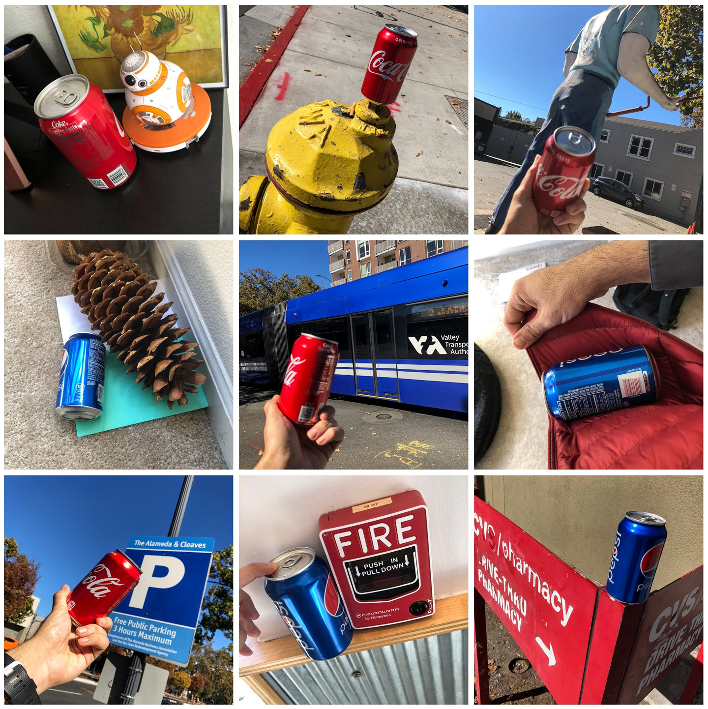
Figure 14-14. Photographs of objects taken in a variety of different settings to train an object detector model
It’s worth taking pictures of the object in environments that it’s unlikely to be used in order to diversify the dataset and improve the robustness of the model. It also has the added bonus of keeping an otherwise boring and tedious process a little entertaining. We can make it interesting by challenging ourselves to come up with unique and innovative photos. Figure 14-15 shows some creative examples of photos taken during the process of building a currency detector.

Figure 14-15. Some creative photographs taken during the process of building a diverse currency dataset
Because we want to make a cat detector, we will be reusing the cat images from the “Cats and Dogs” Kaggle dataset that we used in Chapter 3. We randomly chose images from that set and split them into a train and test set.
To maintain uniformity of input size to our network, we resize all images to a fixed size. We will use the same size as part of our network definition and while converting to a .tflite model. We can use the ImageMagick tool to resize all images at once:
$ apt-get install imagemagick
$ mogrify -resize 800x600 *.jpg
Tip
If you have a large number of images (i.e., several tens of thousands of images) in the current directory, the preceding command might fail to enlist all of the images. A solution would be to use the find command to list all of the images and pipe the output to the mogrify command:
$ find . -type f | awk -F. '!a[$NF]++{print $NF}' |
xargs -I{} mogrify -resize 800x600 *.jpg
Labeling the Data
After we have our data, the next step would be to label it. Unlike classification where simply placing an image in the correct directory would be sufficient, we need to manually draw the bounding rectangles for the objects of interest. Our tool of choice for this task is LabelImg (available for Windows, Linux, and Mac) for the following reasons:
-
You can save annotations either as XML files in PASCAL VOC format (also adopted by ImageNet) or the YOLO format.
-
It supports single and multiclass labels.
Note
If you are the curious cat like us, you’d want to know what the difference is between the YOLO format and the PASCAL VOC format. YOLO happens to use simple .txt files, one per image with the same name, to store information about the classes and the bounding boxes within the image. The following is what a .txt file in YOLO format typically looks like:
class_for_box1 box1_x box1_y box1_w box1_h
class_for_box2 box2_x box2_y box2_w box2_h
Note that the x, y, width, and height in this example are normalized using the full width and height of the image.
PASCAL VOC format, on the other hand, is XML based. Similar to the YOLO format, we use one XML file per image (ideally with the same name). You can view the sample format on the Git repository at code/chapter-14/pascal-voc-sample.xml.
First, download the application from GitHub to a directory on your computer. This directory will have an executable and a data directory containing some sample data. Because we will be using our own custom data, we don’t need the data within the provided data directory. You can start the application by double-clicking the executable file.
At this point, we should have a collection of images that is ready to be used during the training process. We first divide our data randomly into training and test sets and place them in separate directories. We can do this split by simply dragging and dropping the images randomly into either directory. After the train and test directories are created, we load the training directory by clicking Open Dir, as shown in Figure 14-16.

Figure 14-16. Click the Open Dir button and then select the directory that contains the training data
After LabelImg loads the training directory, we can start our labeling process. We must go through each image and manually draw bounding boxes for each object (only cats in our case), as shown in Figure 14-17. After we make the bounding box, we are prompted to provide a label to accompany the bounding box. For this exercise, enter the name of the object, “cat”. After a label is entered, we need only to select the checkbox to specify that label again for subsequent images. For images with multiple objects, we would make multiple bounding boxes and add their corresponding labels. If there are different kinds of objects, we simply add a new label for that object class.

Figure 14-17. Select the Create RectBox from the panel on the left to make a bounding box that covers the cat
Now, repeat this step for all of the training and test images. We want to obtain tight bounding boxes for each object, such that all parts of the object are bounded by the box. Finally, in the train and test directories, we see .xml files accompanying each image file, as depicted in Figure 14-18. We can open the .xml file in a text editor and inspect metadata such as image file name, bounding box coordinates, and label name.

Figure 14-18. Each image is accompanied by an XML file that contains the label information and the bounding box information
Preprocessing the Data
At this point, we have handy XML data that gives the bounding boxes for all of our objects. However, for us to use TensorFlow for training on the data, we must preprocess it into a format that TensorFlow understands, namely TFRecords. Before we can convert our data into TFRecords, we must go through the intermediate step of consolidating the data from all the XML files into a single comma-separated values (CSV) file. TensorFlow provides helper scripts that assist us with these operations.
Now that we have our environment set up, it’s time to begin doing some real work:
-
Convert our cats dataset directory to a single CSV file using the
xml_to_csvtool from the racoon_dataset repository by Dat Tran. We have provided a slightly edited copy of this file in our repository at code/chapter-14/xml_to_csv.py:$ python xml_to_csv.py -i {path to cats training dataset} -o {path to output train_labels.csv} -
Do the same for the test data:
$ python xml_to_csv.py -i {path to cats test dataset} -o {path to test_labels.csv} -
Make the label_map.pbtxt file. This file contains the label and identifier mappings for all of our classes. We use this file to convert our text label into an integer identifier, which is what TFRecord expects. Because we have only one class, the file is rather small and looks as follows:
item { id: 1 name: 'cat' } -
Generate the TFRecord format files that will contain the data to be used for training and testing our model later on. This file is also from the racoon_dataset repository by Dat Tran. We have provided a slightly edited copy of this file in our repository at code/chapter-14/generate_tfrecord.py. (It’s worth noting that the
image_dirpath in the argument should be the same as the path in the XML files; LabelImg uses absolute paths.)$ python generate_tfrecord.py --csv_input={path to train_labels.csv} --output_path={path to train.tfrecord} --image_dir={path to cat training dataset} $ python generate_tfrecord.py --csv_input={path to test_labels.csv} --output_path={path to test.tfrecord} --image_dir={path to cat test dataset}
With our train.tfrecord and test.tfrecord files ready, we can now begin our training process.
Inspecting the Model
(This section is informational only and is not necessary for the training process. You can skip ahead to “Training” if you want to.)
We can inspect our model using the saved_model_cli tool:
$ saved_model_cli show --dir ssd_mobilenet_v2_coco_2018_03_29/saved_model
--tag_set serve
--signature_def serving_default
The output of that script looks like the following:
The given SavedModel SignatureDef contains the following input(s):
  inputs['inputs'] tensor_info:
      dtype: DT_UINT8
      shape: (-1, -1, -1, 3)
      name: image_tensor:0
The given SavedModel SignatureDef contains the following output(s):
  outputs['detection_boxes'] tensor_info:
      dtype: DT_FLOAT
      shape: (-1, 100, 4)
      name: detection_boxes:0
  outputs['detection_classes'] tensor_info:
      dtype: DT_FLOAT
      shape: (-1, 100)
      name: detection_classes:0
  outputs['detection_scores'] tensor_info:
      dtype: DT_FLOAT
      shape: (-1, 100)
      name: detection_scores:0
  outputs['num_detections'] tensor_info:
      dtype: DT_FLOAT
      shape: (-1)
      name: num_detections:0
  outputs['raw_detection_boxes'] tensor_info:
      dtype: DT_FLOAT
      shape: (-1, -1, 4)
      name: raw_detection_boxes:0
  outputs['raw_detection_scores'] tensor_info:
      dtype: DT_FLOAT
      shape: (-1, -1, 2)
      name: raw_detection_scores:0
Method name is: tensorflow/serving/predict
The following is how we can interpret the output from the previous command:
-
The shape of
inputsbeing(-1, -1, -1, 3)indicates that the trained model can accept any arbitrarily sized image input that contains three channels. Due to this inherent flexibility in input size, the converted model would be larger than if the model had a fixed-size input. When we train our own object detector later in this chapter, we will be fixing the input size to 800 x 600 pixels to make the resulting model more compact. -
Moving on to the outputs, the very first output is
detection_boxes (-1, 100, 4). This tells us how many detection boxes are possible, and what will they look like. In particular, the very first number (i.e., -1) indicates that we can have any number of boxes based on the detections for all 100 classes (second number) with four coordinates (third number)—x, y, width, and height—defining each box. In other words, we are not limiting the number of detections for each of the 100 classes. -
For
detection_classes, we have a list of two elements: the first defining how many objects we detected, and the second, a one-hot encoded vector with the detected class enabled. -
num_detectionsis the number of objects detected in the image. It is a single floating point. -
raw_detection_boxesdefines the coordinates of each box that was detected for each object. All of these detections are before the application of NMS on all the detections. -
raw_detection_scoresis a list of two floating-point numbers, the first describing the total number of detections, and the second giving the total number of categories including the background if it is considered a separate category.
Training
Because we are using SSD MobileNetV2, we will need to create a copy of the pipeline.config file (from the TensorFlow repository) and modify it based on our configuration parameters. First, make a copy of the configuration file and search for the string PATH_TO_BE_CONFIGURED within the file. This parameter indicates all of the places that need to be updated with the correct paths (absolute paths preferably) within our filesystem. We will also want to edit some parameters in the configuration file, such as number of classes (num_classes), number of steps (num_steps), number of validation samples (num_examples), and path of label mappings for both the train and test/eval sections. (You’ll find our version of the pipeline.config file on the book’s GitHub website (see http://PracticalDeepLearning.ai).
$ cp object_detection/samples/configs/ssd_mobilenet_v2_coco.config
./pipeline.config
$ vim pipeline.config
Note
In our example, we’re using the SSD MobileNetV2 model to train our object detector. Under different conditions, you might want to choose a different model on which to base your training. Because each model comes with its own pipeline configuration file, you’d be modifying that configuration file, instead. The configuration file comes bundled with each model. You’d use a similar process in which you’d identify the paths that need to be changed and update them using a text editor accordingly.
In addition to modifying paths, you might want to modify other parameters within the configuration file such as image size, number of classes, optimizer, learning rate, and number of epochs.
So far, we’ve been at the models/research directory within the TensorFlow repository. Let’s now move into the object_detection directory and run the model_main.py script from TensorFlow, which trains our model based on the configuration provided by the pipeline.config file that we just edited:
$ cd object_detection/
$ python model_main.py
--pipeline_config_path=../pipeline.config
--logtostderr
--model_dir=training/
We’ll know the training is happening correctly when we see lines of output that look like the following:
Average Precision (AP) @[ IoU=0.50:0.95 | area=all | maxDets=100 ] = 0.760
Depending on the number of iterations that we are training for, the training will take from a few minutes to a couple of hours, so plan to have a snack, do the laundry, clean the litter box, or better yet, read the chapter ahead. After the training is complete, we should see the latest checkpoint file in the training/ directory. The following files are also created as a result of the training process:
$ ls training/

checkpoint                                   model.ckpt-13960.meta
eval_0                                       model.ckpt-16747.data-00000-of-00001
events.out.tfevents.1554684330.computername  model.ckpt-16747.index
events.out.tfevents.1554684359.computername  model.ckpt-16747.meta
export                                       model.ckpt-19526.data-00000-of-00001
graph.pbtxt                                model.ckpt-19526.index
label_map.pbtxt                            model.ckpt-19526.meta
model.ckpt-11180.data-00000-of-00001       model.ckpt-20000.data-00000-of-00001
model.ckpt-11180.index                     model.ckpt-20000.index
model.ckpt-11180.meta                      model.ckpt-20000.meta
model.ckpt-13960.data-00000-of-00001       pipeline.config
model.ckpt-13960.index
We convert the latest checkpoint file to the .TFLite format in the next section.
Tip
Sometimes, you might want to do a deeper inspection of your model for debugging, optimization, and/or informational purposes. Think of it like a DVD extra of a behind-the-scenes shot of your favorite TV show. You would run the following command along with arguments pointing to the checkpoint file, the configuration file, and the input type to view all the different parameters, the model analysis report, and other golden nuggets of information:
$ python export_inference_graph.py
--input_type=image_tensor
--pipeline_config_path=training/pipeline.config
--output_directory=inference_graph
--trained_checkpoint_prefix=training/model.ckpt-20000
The output from the this command looks like the following:
=========================Options=========================
-max_depth                  10000
-step                       -1
...

==================Model Analysis Report==================
...
Doc:
scope: The nodes in the model graph are organized by
their names, which is hierarchical like filesystem.
param: Number of parameters (in the Variable).

Profile:
node name | # parameters
_TFProfRoot (--/3.72m params)
 BoxPredictor_0 (--/93.33k params)
    BoxPredictor_0/BoxEncodingPredictor
    (--/62.22k params)
      BoxPredictor_0/BoxEncodingPredictor/biases
      (12, 12/12 params)
 ...
FeatureExtractor (--/2.84m params)
...
This report helps you to learn how many parameters you have, which could in turn help you in finding opportunities for model optimization.
Model Conversion
Now that we have the latest checkpoint file (the suffix should match the number of epochs in the pipeline.config file), we will feed it into the export_tflite_ssd_graph script like we did earlier in the chapter with our pretrained model:
$ python export_tflite_ssd_graph.py
--pipeline_config_path=training/pipeline.config
--trained_checkpoint_prefix=training/model.ckpt-20000
--output_directory=tflite_model
--add_postprocessing_op=true
If the preceding script execution was successful, we’ll see the following files in the tflite_model directory:
$ ls tflite_model
tflite_graph.pb
tflite_graph.pbtxt
We have one last step remaining: convert the frozen graph files to the .TFLite format. We can do that using the tflite_convert tool:
$ tflite_convert --graph_def_file=tflite_model/tflite_graph.pb
--output_file=tflite_model/cats.tflite
--input_arrays=normalized_input_image_tensor
--output_arrays='TFLite_Detection_PostProcess','TFLite_Detection_PostProcess:1','TFLi
te_Detection_PostProcess:2','TFLite_Detection_PostProcess:3'
--input_shape=1,800,600,3
--allow_custom_ops
In this command, notice that we’ve used a few different arguments that might not be intuitive at first sight:
-
For
--input_arrays, the argument simply indicates that the images that will be provided during predictions will be normalizedfloat32tensors. -
The arguments supplied to
--output_arraysindicate that there will be four different types of information in each prediction: the number of bounding boxes, detection scores, detection classes, and the coordinates of bounding boxes themselves. This is possible because we used the argument--add_postprocessing_op=truein the export graph script in the previous step. -
For
--input_shape, we provide the same dimension values as we did in the pipeline.config file.
The rest are fairly trivial. We should now have a spanking new cats.tflite model file within our tflite_model/ directory. It is now ready to be plugged into an Android, iOS, or edge device to do live detection of cats. This model is well on its way to saving Bob’s garden!
Tip
In the floating-point MobileNet model, 'normalized_image_tensor' has values between [-1,1). This typically means mapping each pixel (linearly) to a value between [–1,1]. Input image values between 0 and 255 are scaled by (1/128) and then a value of –1 is added to them to ensure the range is [-1,1).
In the quantized MobileNet model, 'normalized_image_tensor' has values between [0, 255].
In general, see the preprocess function defined in the feature extractor class in the TensorFlow Models repository at models/research/object_detection/models directory.
Image Segmentation
Taking a step further beyond object detection, to get more precise locations of objects, we can perform object segmentation. As we saw earlier in this chapter, this involves making category predictions for each pixel in an image frame. Architectures such as U-Net, Mask R-CNN, and DeepLabV3+ are commonly used to perform segmentation tasks. Similar to object detection, there has been a growing trend of running segmentation networks in real time, including on resource-constrained devices such as smartphones. Being real time opens up many consumer app scenarios like face filters (Figure 14-19), and industrial scenarios such as detecting drivable roads for autonomous cars (Figure 14-20).

Figure 14-19. Colorizing hair with ModiFace app by accurately mapping the pixels belonging to the hair

Figure 14-20. Image segmentation performed on frames from a dashcam (CamVid dataset)
As you might have grown accustomed to hearing in this book by now, you can accomplish much of this without needing much code. Labeling tools like Supervisely, LabelBox, and Diffgram can help not just label the data, but also load previously annotated data and train further on a pretrained object segmentation model. Moreover, these tools provide AI-assisted labeling, which can dramatically speed up (~10 times) the otherwise laborious and expensive labeling process. If this sounds exciting, you are in luck! We have included a bonus resource guide on how to learn and build segmentation projects on the book’s GitHub website (see http://PracticalDeepLearning.ai).
Case Studies
Let’s now look at how object detection is being used to power real-world applications in the industry.
Smart Refrigerator
Smart fridges have been gaining popularity for the past few years because they have started to become more affordable. People seem to like the convenience of knowing what’s in their fridge even when they are not home to look inside. Microsoft teamed up with Swiss manufacturing giant Liebherr to use deep learning in its new generation SmartDeviceBox refrigerator (Figure 14-21). The company used Fast R-CNN to perform object detection within its refrigerators to detect different food items, maintain an inventory, and keep the user abreast of the latest state.

Figure 14-21. Detected objects along with their classes from the SmartDeviceBox refrigerator (image source)
Crowd Counting
Counting people is not just something that only cats do while staring out of windows. It’s useful in a lot of situations including managing security and logistics at large sporting events, political gatherings, and other high-traffic areas. Crowd counting, as its name suggests, can be used to count any kind of object including people and animals. Wildlife conservation is an exceptionally challenging problem because of the lack of labeled data and intense data collection strategies.
Wildlife conservation
Several organizations, including the University of Glasgow, University of Cape Town, Field Museum of Natural History, and Tanzania Wildlife Research Institute, came together to count the largest terrestrial animal migration on earth: 1.3 million blue wildebeest and 250,000 zebra between the Serengeti and the Masaai Mara National Reserve, Kenya (Figure 14-22). They employed data labeling through 2,200 volunteer citizen scientists using a platform called Zooniverse and used automated object detection algorithms like YOLO for counting the wildebeest and zebra population. They observed that the count from the volunteers and from the object detection algorithms were within 1% of each other.

Figure 14-22. An aerial photograph of wildebeest taken from a small survey airplane (image source)
Kumbh Mela
Another example of dense crowd counting is from Prayagraj, India where approximately 250 million people visit the city once every 12 years for the Kumbh Mela festival (Figure 14-23). Crowd control for such large crowds has historically been difficult. In fact, in the year 2013, due to poor crowd management, a stampede broke out tragically resulting in the loss of 42 lives.
In 2019, the local state government contracted with Larsen & Toubro to use AI for a variety of logistical tasks including traffic monitoring, garbage collection, security assessments, and also crowd monitoring. Using more than a thousand CCTV cameras, authorities analyzed crowd density and designed an alerting system based on the density of people in a fixed area. In places of higher density, the monitoring was more intense. It made the Guinness Book of World Records for being the largest crowd management system ever built in the history of humankind!

Figure 14-23. The 2013 Kumbh Mela, as captured by an attendee (image source)
Face Detection in Seeing AI
Microsoft’s Seeing AI app (for the blind and low-vision community) provides a real-time facial detection feature with which it informs the user of the people in front of the phone’s camera, their relative locations, and their distance from the camera. A typical guidance might sound like “One face in the top-left corner, four feet away.” Additionally, the app uses the facial-detection guidance to perform facial recognition against a known list of faces. If the face is a match, it will announce the name of the person, as well. An example of vocal guidance would be “Elizabeth near top edge, three feet away,” as demonstrated in Figure 14-24.
To identify a person’s location in the camera feed, the system is running on a fast mobile-optimized object detector. A crop of this face is then passed for further processing to age, emotion, hair style, and other recognition algorithms on the cloud from Microsoft’s Cognitive Services. For identifying people in a privacy-friendly way, the app asks the user’s friends and family to take three selfies of their faces and generates a feature representation (embedding) of the face that is stored on the device (rather than storing any images). When a face is detected in the camera live feed in the future, an embedding is calculated and compared with the database of embeddings and associated names. This is based on the concept of one-shot learning, similar to Siamese networks that we saw in Chapter 4. Another benefit of not storing images is that the size of the app doesn’t increase drastically even with a large number of faces stored.

Figure 14-24. Face detection feature on Seeing AI
Autonomous Cars
Several self-driving car companies including Waymo, Uber, Tesla, Cruise, NVIDIA, and others use object detection, segmentation, and other deep learning techniques for building their self-driving cars. Advanced Driver Assistance Systems (ADAS) such as pedestrian detection, vehicle type identification, and speed limit sign recognition are important components of a self-driving car.
For the decision-making involved in self-driving cars, NVIDIA uses specialized networks for different tasks. For example, WaitNet is a neural network used for doing fast, high-level detection of traffic lights, intersections, and traffic signs. In addition to being fast, it is also meant to withstand noise and work reliably in tougher conditions such as rain and snow. The bounding boxes detected by WaitNet are then fed to specialized networks for more detailed classification. For instance, if a traffic light is detected in a frame, it is then fed into LightNet—a network used for detecting traffic light shape (circle versus arrow) and state (red, yellow, green). Additionally, if a traffic sign is detected in a frame, it’s fed into SignNet, a network to classify among a few hundred types of traffic signs from the US and Europe, including stop signs, yield signs, directional information, speed limit information, and more. Cascading output from faster networks to specialized networks helps improve performance and modularize development of different networks.

Figure 14-25. Detecting traffic lights and signs on a self-driving car using the NVIDIA Drive Platform (image source)
Summary
In this chapter, we explored the types of computer-vision tasks, including how they relate to one another and how they are different from one another. We took a deeper look at object detection, how the pipeline works, and how it evolved over time. We then collected data, labeled it, trained a model (with and without code), and deployed the model to mobile. We next looked at how object detection is being used in the real world by industry, government, and non-governmental organizations (NGOs). And then we took a sneak peek into the world of object segmentation. Object detection is a very powerful tool whose vast potential is still being discovered every day in numerous areas of our lives. What innovative use of object detection can you think of? Share it with us on Twitter @PracticalDLBook.