
14 2. BASICS OF FEATURE DESIGN
density estimator in a regular grid [Felsberg et al., 2006]. e mathematical proof has basically
already been given in the context of averaged shifted histograms by Scott [1985].
In the work mentioned in the previous paragraph, channel coding is applied to the feature
domain, i.e., as a histogram approach. Obviously, it can also be applied to the spatial domain, i.e.,
as a signature approach. Combining both results in CCFM [Jonsson and Felsberg, 2009]. Both
SIFT and HOG descriptors can be considered as a particular variants of CCFMs, as will be
shown in Chapter 4. e CCFM framework allows generalizing to color images [Felsberg and
Hedborg, 2007a] and its mathematical basis in frame theory enables a decoding methodology,
which also includes visual reconstruction [Felsberg, 2010]; see Chapter 5.
Channel representations have originally been proposed based on a number of properties
(non-negativity, locality, smoothness; Granlund [2000b]). ese properties together with the
invariance requirement for the L
2
-norm of regularly placed channels [Nordberg et al., 1994]
imply the frame properties of channel representation [Forssén, 2004] and the uniqueness of
the cos
2
-basis function [Felsberg et al., 2015]. Irregular placement of channels, as suggested
by Granlund [2000b], obviously does not result in such a stringent mathematical framework,
but is particularly powerful for image analysis using machine learning and the representation of
less structured spaces, such as color. In that sense, color names [Van De Weijer et al., 2009] can
be understood as a non-regular spaced channel representation.
Similar to RGB color-space and intensity space, the non-negativity constraint for channel
representations implies a non-Euclidean geometry. More concretely, the resulting coefficient
vector lies in a multi-dimensional cone and transformations on those vectors are restricted to be
hyperbolic [Lenz et al., 2007]. is also coincides with observations made by Koenderink and
van Doorn [2002] that Euclidean transformations of image space (spatio-intensity space) are
inappropriate for image analysis.
A further conclusion is that the L
2
-distance is inappropriate to measuring distances in
these non-negative spaces. Still, many applications within image analysis and machine learning
are based on the L
2
-distance. More suitable alternatives, based on probabilistic modeling, are
discussed in Chapter 6.
2.5 LINKS TO BIOLOGICALLY INSPIRED MODELS
As mentioned in the previous sections, channel representations originate mainly from technical
requirements and principles, but were also inspired by biology [Granlund, 1999]. ey share
many similarities with population codes in computational neuroscience [Lüdtke et al., 2002,
Pouget et al., 2003], which are conversely mainly motivated by observations in biological sys-
tems.
To complete confusion, the concept of population codes developed historically from ap-
proaches that used the term “channel codes” [Snippe and Koenderink, 1992]. Channel (or pop-
ulation) codes have been suggested repeatedly as a computational model for observations in
human perception and cognition.
2.5. LINKS TO BIOLOGICALLY INSPIRED MODELS 15
e term “channel” has also been used by Howard and Rogers [1995], writing about
sensory channels that establish labeled-line detectors, which have a bandpass tuning function. e
activation of these detectors happens through bell-shaped sensitivity curves and controls the
frequency of firing.
e observation of firing rates in biological systems also inspired the approach of asyn-
chronous networks based on spikes, the spikenets, proposed by orpe [2002]. e simple mech-
anisms, and in particular the non-negative nature of frequency, enables high-speed computa-
tions on low-resource systems.
However, activation-level-based, synchronous networks are more suitable for digital com-
puters, including modern GPU-based systems, and thus most computational models for popu-
lation codes. Intensity-based systems need different mechanisms than those based on sequences
of spikes, but require regularization and enforcement of non-negativity.
e regularization of the number of active coefficients (or their L
1
-norm) leads to the
concept of sparse coding [Olshausen and Field, 1997]. Such systems are naturally robust and
require few computations. Another regularization option is by means of continuity, resulting in
the predictive coding paradigm [Rao and Ballard, 1999]. Also, this approach helps to design
robust systems with low computational demand.
A further concern in coding systems is the design of an unbiased readout, i.e., no value-
dependent systematic error occurs in the decoding [Denève et al., 2001]. e proposed iterative
algorithm for the readout of population codes [Denève et al., 1999] is very similar to the newly
published routing algorithm in deep networks [Sabour et al., 2017], but, as we will show in
Chapter 5, not really unbiased.
Besides individual coding aspects, structural and topological knowledge from biological
observation also are exploited in the design of systems, see e.g., the work by Riesenhuber and
Poggio [1999]. Most of these works are to some extent based on the pioneering work of Hubel
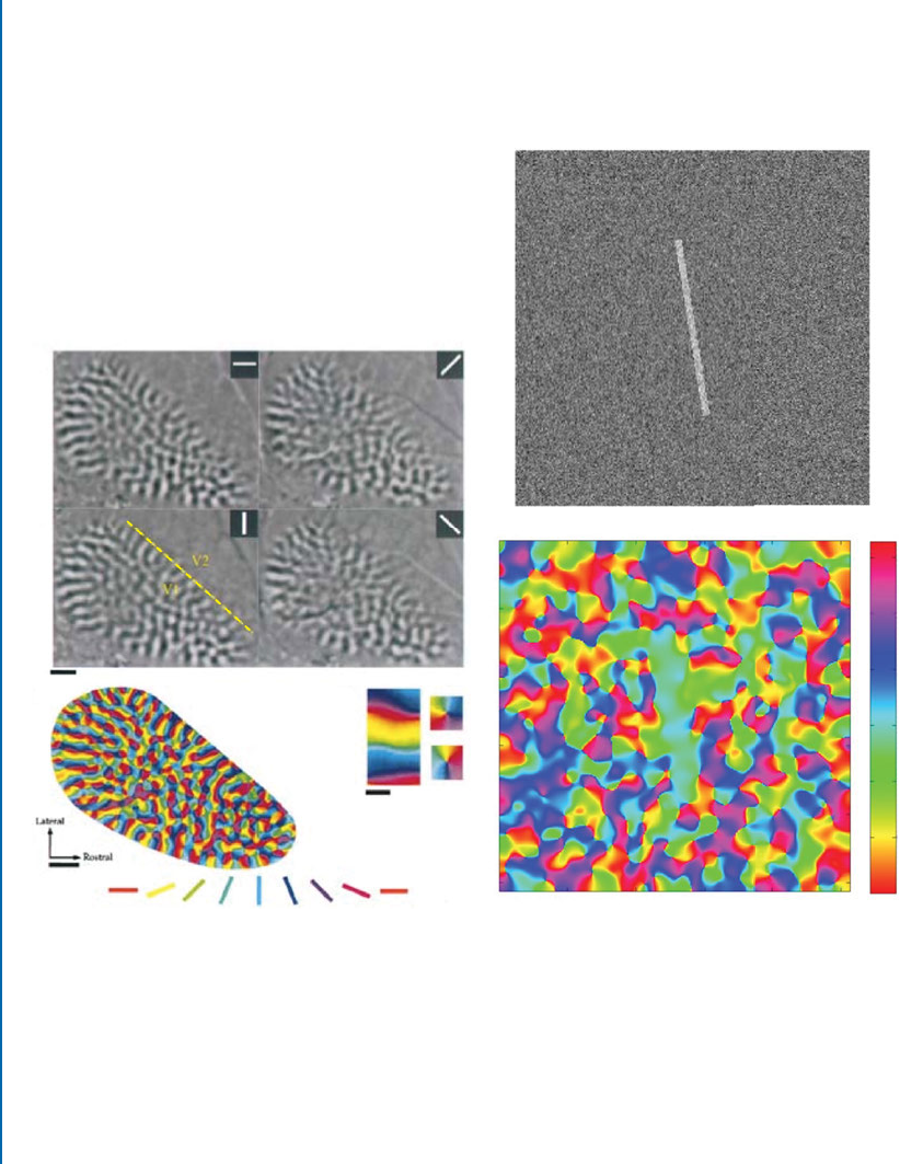
and Wiesel [1959]. Channel representations are no exception here as can be observed in Fig-
ure 2.4. e right-hand illustration has been generated with the channel representation and
shares many similarities with the left part of the figure.
SUMMARY
In this chapter we have given a short overview of statistical design principles for visual features,
invariance/equivariance properties, sparse and compact representations, histograms, and signa-
tures. We have provided a brief survey of the most important grid-based feature representations
that are relevant to channel representations and CCFMs. Finally, we have related the chan-
nel representation to a number of approaches mainly inspired from biology. In the subsequent
chapter we will now focus on the technical details of channel encoding, reflecting also on the
relations to other feature extraction methods in more detail.
16 2. BASICS OF FEATURE DESIGN
A
D
B C
E
V2
V1
1mm
1mm
200 µm
50
100
150
200
250
50 100 150 200 250
3
2.5
2
1.5
1
0.5
Figure 2.4: Left: reproduced with permission from Bosking et al. [1997]. A: parts of visual cortex
active under orientation stimuli. B: orientation map obtained by vector summation. Right: figure
from Felsberg et al. [2015]. D: stimulus. E: response from channel smoothing of orientation.
..................Content has been hidden....................
You can't read the all page of ebook, please click here login for view all page.