

26 3. CHANNEL CODING OF FEATURES
where denotes the convolution (thus scalar products over all translations), R
˛
a rotation by ˛,
and the kernel of the orientation score, the wavelet.
In order to enable well-posed reconstruction, must fulfill an energy constraint based on
M
.u; v/ D
1
N
N 1
X
nD0
jF .R
2 n=N
/.u; v/j
2
; (3.24)
where F denotes the Fourier transform from .i; j / to .u; v/.
If M
D 1, the original function x can by reconstructed as
Qx.i; j / D
N 1
X
n
D
0
U
N
x
.i; j; n/ : (3.25)
Orientation scores can also be extended to the similitude group, as suggested by Sharma
and Duits [2015]. e approach is very similar to calculating a channel representation in the
log-polar domain, see e.g., Öäll and Felsberg [2017]. For this approach, multi-dimensional
channel coding is required.
3.4 MULTI-DIMENSIONAL CODING
In previous sections, only one-dimensional random variables x have been considered. e chan-
nel coefficients that are obtained by coding one-dimensional variables are basically stochastically
independent, except for those with overlapping kernels, i.e., the two neighbors in case of cos
2
-
kernels. In the subsequent considerations in this section, the effect of the overlapping kernels
is ignored and all coefficients are considered independent, which is strictly true only for the
rectangular kernel.
If multi-dimensional random vectors with independent components are encoded, all di-
mensions can be encoded and stored independently. After summing over all observed samples,
the densities of the marginal distributions are obtained and since those are independent, an
estimate of the joint estimate is obtained by multiplying these marginal estimates. For two-
dimensional samples .x
1
; x
2
/ with channel coefficients .c
1;n
1
; c
2;n
2
/, we obtain by (3.15)
EŒc
1;n
1
EŒc
2;n
2
D
Z
p.x
1
/K.x
1
1;n
1
/ dx
1
Z
p.x
2
/K.x
2
2;n
2
/ dx
2
(3.26)
D
“
p.x
1
; x
2
/K.x
1
1;n
1
/K.x
2
2;n
2
/ dx
1
dx
2
(3.27)
D EŒc
1;n
1
c
2;n
2
: (3.28)
One such case is color and orientation in a local region, see Figure 3.7.
In general, one might assume that color and orientation are mutually independent and
the joint distribution can be computed by multiplying the marginal distributions of color and
orientation.

3.4. MULTI-DIMENSIONAL CODING 27
Figure 3.7: Simultaneous encoding of color and orientation in a local image region. Figure taken
from Jonsson [2008] courtesy Erik Jonsson. e red circle on the left indicates the considered
local region and the color and orientation patterns on the right represent the channels of the
marginal distributions. In the present example, color and orientation are not completely inde-
pendent, such that the channel matrix, represented by the black blobs, cannot be factorized.
If the components of the random vector are not mutually independent, for instance be-
cause the observed objects, such as bananas or skyscrapers, lead to color-dependent orientation
distributions, the identity leading to (3.27) breaks. is effect has also been observed in the case
of texture classification by Khan et al. [2013].
In the general case, the expectation of the product of channel coefficients can thus not be
computed from the product of their expectations,
EŒc
1;n
1
EŒc
2;n
2
¤ EŒc
1;n
1
c
2;n
2
; (3.29)
implying that summation over the sample index must happen after the outer product of channel
vectors.
One such example are optical flow vectors, where moving edges and lines have highly cor-
related spatial displacements [Spies and Forssén, 2003]. Obviously, this leads to an exponential
growth of the number of coefficients with the number of dimensions. If all d dimensions are
encoded with the same number of channels N , the total number of coefficients becomes N
d
.
In practice, however, this is seldom a problem. In many cases, not all product terms stem-
ming from the outer products are required, e.g., Granlund [2000b] suggests to only use second
order terms, or the mutual dependency can be ignored altogether without compromising the
results [Wallenberg et al., 2011].
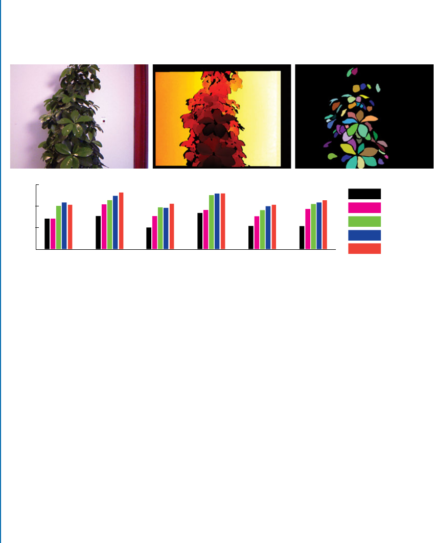
In the latter work, RGB color and depth gradients (D), which both have a two-
dimensional correlation structure, are channel coded and concatenated. is approach leads
to improved segmentation performance, see Figure 3.8. Presumably, the segmentation perfor-
28 3. CHANNEL CODING OF FEATURES
mance could be further improved by replacing RGB values with color names, the previously
mentioned 11-dimensional learned soft-assignment suggested by Van De Weijer et al. [2009]
that shares also similarities to channel representations, but this pathway has not been further
explored.
Plant6Plant5P
lant4Plant3*Plant2Plant1*
Score
Depth
Color
∆depth
RGB+∆D
CC RGB+∆D
0.75
0.5
0.25
0
Figure 3.8: Top from left to right: plant 5 from the plant data set (Wallenberg et al. [2011])
RGB, depth, and ground truth segmentation. Bottom: consensus scores by various feature com-
binations. Images indicated with asterisks were used for parameter tuning of all compared meth-
ods. Note that although RGBCD and channel-coded RGBCD have similar results on the
tuning images, channel-coded RGBCD has a higher score on all evaluation images.
Even if all possible combinations of channel coefficients are taken into account, the total
number of non-zero products has an upper bound which is linear in the number of observed
samples as observed by Felsberg and Granlund [2006].
In that work, three performance experiments have been conducted where a number M
of samples in spaces of dimension d D 1 : : : 9 have been encoded with N channels in each di-
mension, see Figure 3.9. e comparison of time consumption for M D 5;000 and M D 10;000
samples and N D 10 shows a proportional increase with the number of samples. e comparison
of N D 10 and N D 20 for M D 10;000 samples shows no increase of time consumption. us,
if sparse data structures are used to store the coefficient matrices, a brute-force outer product
of all dimensions is feasible and still allows for real-time performance [Felsberg and Hedborg,
2007b, Pagani et al., 2009].
Interestingly, the absence of observations for most of the products gets completely dif-
ferent meanings in a frequentist and a bayesian interpretation: e former simply assumes zero
probability, whereas the latter computes a non-zero probability depending on the assumed prior

3.4. MULTI-DIMENSIONAL CODING 29
987654321
0
0.1
0.2
0.3
0.4
Figure 3.9: Time consumption for encoding, implemented in Matlab on a Powerbook with
1 GHz PPC. Ordinate: dimensions d D 1 : : : 9, abscissa: time in seconds (averaged over 10
runs). Dashed line: 5,000 samples, 10
d
channels. Solid line: 10,000 samples, 10
d
channels. Dot-
ted line: 10,000 samples, 20
d
channels. Figure from Felsberg and Hedborg [2007b].
(e.g., a Dirichlet distribution, see also Chapter 6) and the total number of observations falling
into other bins. However, in either case, the estimate for the density can be computed from the
sparse data structure.
With the introduction of P-channels [Felsberg and Granlund, 2006] a computationally
more efficient approximation to compute linear B-spline kernels has been introduced. Besides
the computational considerations, also explicit spatial pooling has been suggested.
Instead of computing local averages over image regions and maintaining the image res-
olution, as e.g., suggested by Felsberg and Granlund [2003], the channel representations are
simultaneously low-pass filtered and down-sampled, reducing the computational effort further.
is spatial pooling is explicit, because the local coordinates are also considered as part of the
random vector. e vector now contains a part with spatial coordinates and a feature part, to-
gether forming the spatio-featural space proposed by Jonsson and Felsberg [2009]. is approach
will be further considered in the subsequent chapter.
SUMMARY
In this chapter we have introduced the channel encoding of visual features. e resulting rep-
resentation is an efficient approximation of a kernel density estimator for the distribution of
the encoded features. We have related the approach to population coding, DFs, and orientation
scores. In the subsequent chapter we will now focus on spatial maps of channel encoded features,
i.e., CCFMs and their relation to popular 2D features such as SIFT and HOG and 3D features
such as SHOT.
..................Content has been hidden....................
You can't read the all page of ebook, please click here login for view all page.