

57
C H A P T E R 6
Probabilistic Interpretation of
Channel Representations
e channel representation was originally introduced as a deterministic information represen-
tation concept, based on methods from signal processing and motivated by observation from
biology (Granlund [2000b], Section 2.5). Due to its relation to histograms and kernel den-
sity estimators, connections to probabilistic interpretations have been identified in later years
by Felsberg et al. [2006] and Duits, Felsberg, Granlund and ter Haar Romeny [2007].
In particular, the distribution of coefficient values can be considered in context of multi-
nomial distributions and their divergences, also leading to a connection with categorical distri-
butions and thus symbolic (discrete) spaces. Finally, concepts like stochastic independence and
Copulas are considered.
6.1 ON THE DISTRIBUTION OF CHANNEL VALUES
Starting from the observation of channel representations being soft histograms, see Section 2.4,
we build the subsequent consideration on the statistics of histograms, i.e., channel representa-
tions with rectangular kernels (3.2). Each of the bins corresponds to counting the appearance of
an event, namely the value falling inside of a certain interval.
If we now assume that the event for each bin has a certain probability P
n
0 such that
P
N
nD1
P
n
D 1 and that the events of choosing bins are independent, we obtain a multinomial
distribution with parameters M (the number of trials) and P D .P
1
; : : : ; P
N
/; see Evans et al.
[2000].
From the literature we know that the expectation of histogram bin/channel coefficient c
n
is given as
EŒc
n
D MP
n
(6.1)
and (co-)variances of bins/channels are
varŒc
n
D MP
n
.1 P
n
/ covŒc
n
; c
n
0
D MP
n
P
n
0
: (6.2)
us, for large numbers of trials, the normalized channel coefficients c
n
=M can be used as ap-
proximate estimates of the probabilities. e variance is minimal for extreme cases (very small
or very large coefficients) and covariances are always negative, meaning that if a trials falls into
one bin, the expectation for the other bins is reduced.
58 6. PROBABILISTIC INTERPRETATION OF CHANNEL REPRESENTATIONS
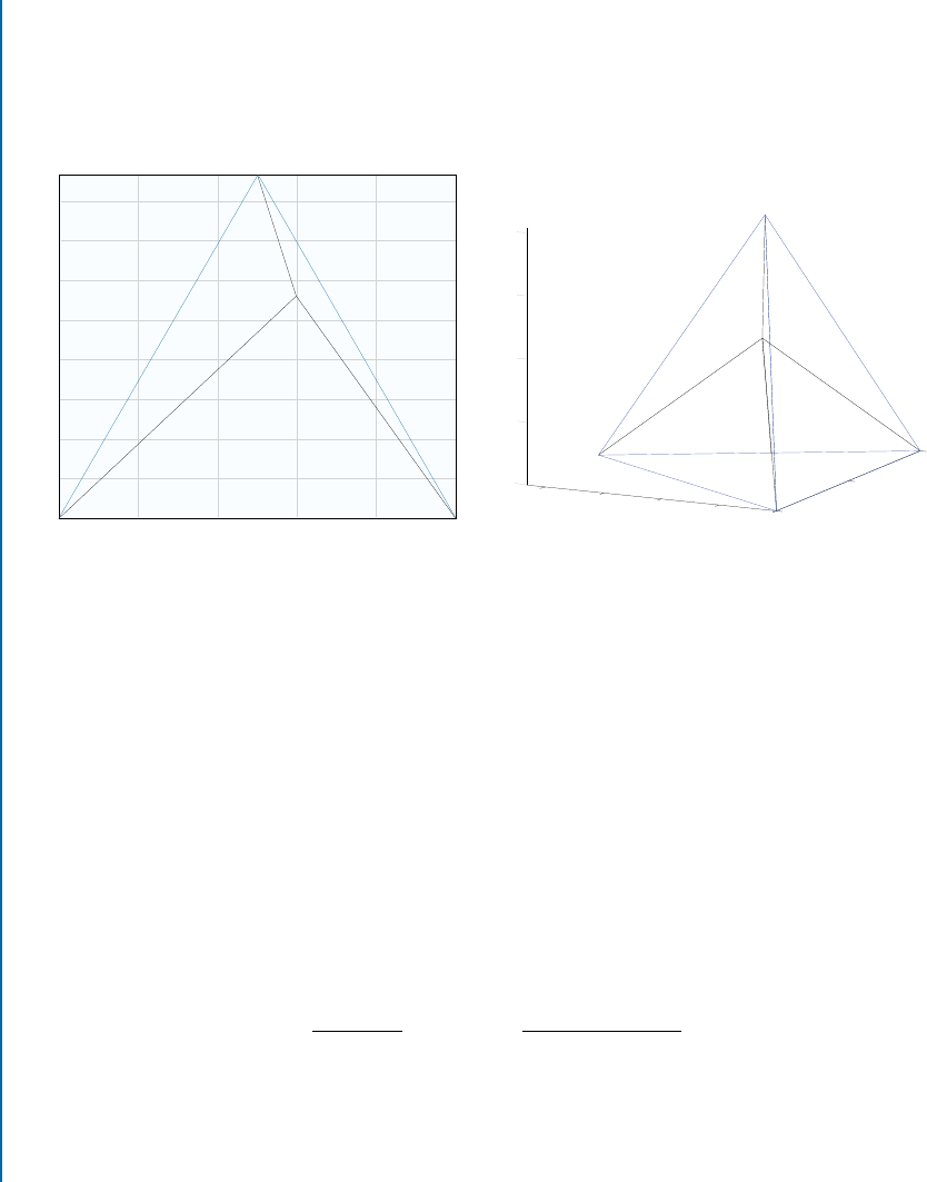
Interestingly, there is geometric interpretation of multinomial distributions in terms of
(generalized) barycentric coordinates, i.e., multi-dimensional equilateral pyramids; see Fig-
ure 6.1. e cases of small variance are those close to the corners of the pyramid, closely related
to the case of distinct intrinsic dimensionality in Felsberg et al. [2009]. e pyramidal structure
stems from the fact that P is an element of the probability simplex S
N
.
0 10.2 0.4 0.6 0.8
0
0.1
0.2
0.3
0.4
0.5
0.6
0.7
0.8
c
3
c
2
c
1
c
1
0
0.5
1
0
0.2
0.4
0.6
0.8
0
0.2
0.4
0.6
0.8
c
3
c
4
c
2
Figure 6.1: Illustration of multidimensional simplexes in 2D and 3D. e 1D simplex is just
the interval Œ0I1 on the real line. e 2D simplex is what is commonly called barycentric co-
ordinates, a triangle parametrized by three values .c
1
; c
2
; c
3
/ with unit sum. In 3D, we obtain a
tetrahedron, parametrized with four values .c
1
; : : : ; c
4
/. Higher-dimensional cases can be illus-
trated only as animations, e.g., 4D simplex http://liu.diva-portal.org/smash/get/div
a2:916645/MOVIE02.mp4.
e likelihood to observe the channel vector
c
is given by drawing
M D
N
X
nD1
c
n
(6.3)
samples and distribute them in the N bins, see Evans et al. [2000],
p.cjP; M / D
M Š
Q
N
n
D
1
c
n
Š
N
Y
nD1
P
c
n
n
D
.M C 1/
Q
N
n
D
1
.c
n
C 1/
N
Y
nD1
P
c
n
n
; (6.4)
where the Gamma function
.s/ D
Z
1
0
t
s1
exp.t/ dt s 2 R
C
(6.5)

6.1. ON THE DISTRIBUTION OF CHANNEL VALUES 59
is the continuous generalization of the factorial function .s 1/Š for s 2 N.
Obviously, we are interested in the posterior rather than the likelihood and therefore we
also have to consider the prior of the multinomial distribution. e conjugate prior of the multi-
nomial distribution is the Dirichlet distribution
p.P/ D Dir.Pj˛
˛
˛/ D
.
P
N
nD1
˛
n
/
Q
N
nD1
.˛
n
/
N
Y
nD1
P
˛
n
1
n
; (6.6)
where the concentration parameters ˛
˛
˛ D .˛
1
; : : : ; ˛
N
/ are positive reals and small values prefer
sparse distributions [Hutter, 2013]. Since we do not have a reason to assume different initial
concentrations for different bins, we consider the symmetric Dirichlet distribution as prior, i.e.,
˛
1
D : : : D ˛
N
D ˛,
Dir.Pj˛/ D
.˛N /
.˛/
N
N
Y
nD1
P
˛1
n
: (6.7)
us, the posterior distribution p.Pjc/ is proportional to
p.cjP/Dir.Pj˛/ D
.M C 1/
Q
N
nD1
.c
n
C 1/
N
Y
nD1
P
c
n
n
.˛N /
.˛/
N
N
Y
nD1
P
˛1
n
(6.8)
D
.M C 1/
Q
N
nD1
.c
n
C 1/
.
P
N
nD1
˛/
Q
N
nD1
.˛/
N
Y
nD1
P
c
n
C˛1
n
(6.9)
/
.
P
N
nD1
c
n
C ˛/
Q
N
nD1
.c
n
C ˛/
N
Y
nD1
P
c
n
C˛1
n
(6.10)
D Dir.Pjc C ˛/ ; (6.11)
and the posterior distribution is a Dirichlet distribution with concentration parameter vector c C
˛. e posterior distribution is useful as it allows to compute divergences between histograms
in statistically correct sense, from a Bayesian point of view; see Section 6.3.
From the posterior distribution we can compute the posterior predictive p.c
0
jc/ by in-
tegrating the product of likelihood and posterior distribution over the probability simplex S
N
,
resulting in a predicted histogram; see Section 6.2.
Finally, by integrating the posterior distribution over the probability simplex S
N
, we ob-
tain the marginal distribution of the data, relevant for determining the correct Copula (in a
Bayesian sense); see Section 6.4.
So far, we have only been considering histograms, i.e., rectangular kernel functions. Fol-
lowing the arguments of Scott [1992], the same statistical properties are obtained for linear
interpolation between histogram bins. In the most general case, however, and in particular for
the most useful kernels such as cos
2
, the correlation between neighbored bins violates the as-
sumption about independent events for the respective bins.
..................Content has been hidden....................
You can't read the all page of ebook, please click here login for view all page.