

64 6. PROBABILISTIC INTERPRETATION OF CHANNEL REPRESENTATIONS
Similarly, we can compute a closed form solution for the Hellinger divergence of Dirichlet
distributions
H
˛
.p.Pjc/kp.Pjc
0
// D
1
˛ 1
B.c
0
/
˛1
B.c
˛
/
B.c/
˛
1
; (6.26)
but for numerical reasons, the Rényi divergence is preferable as it can be computed using log-
Beta functions betaln./
R
˛
.p.Pjc/kp.Pjc
0
// D betaln.c
0
/ C
1
˛ 1
betaln.c
˛
/
˛
˛ 1
betaln.c/ : (6.27)
A further reason to prefer Rényi divergence over Hellinger divergence is the respective sensitivity
to small perturbations. e derivative of the Hellinger divergence with respect to single channel
coefficients scales with the divergence itself, which leads to a lack of robustness. In contrast,
@R
˛
.p.Pjc/kp.Pjc
0
//
@c
0
n
D .c
0
n
/ .jc
0
j/ C .jc
˛
j/ .c
˛;n
/ ; (6.28)
where .c
n
/ D
0
.c
n
/
.c
n
/
is the digamma function, see, e.g., Van Trees et al. [2013, p. 104].
us, the Rényi divergences of the posteriors estimated from c and c
0
are candidates for
suitable distance measures. Unfortunately, robustness against outliers is still limited and the
introduction of an outlier process as in (6.25) is analytically cumbersome.
Also, the fully symmetric setting is less common in practice, but occurs, e.g., in the com-
putation of affinity matrices for spectral clustering. Most cases aim at the comparison of a new
measurement with previously acquired ones and the posterior predictive (6.25) is more suitable.
e proposed distances have been discussed assuming one-dimensional distributions, but
the results generalize to higher dimensions, both for independent and dependent stochastic
variables. Obviously, it is an advantage to have uniform marginals and for that case, dependent
joint distributions correspond to a non-constant Copula distribution; see Section 6.4.
6.4 UNIFORMIZATION AND COPULA ESTIMATION
As mentioned in Section 6.1, we often assume a uniform prior for the channel vector. However,
if we compute the marginal distribution from the posterior distribution for a large dataset, the
components of a channel vector might be highly unbalanced. is issue can be addressed by
placing channels in a non-regular way, according to the marginal distribution, i.e., with high
channel density where samples are likely.
is placement is obtained by mapping samples using the cumulative density function of
the distribution from which the samples are drawn. e cumulative density can be computed
from the estimated distribution as obtained from maximum entropy decoding; see Section 5.3.
e subsequent procedure has been proposed by Öäll and Felsberg [2017].

6.4. UNIFORMIZATION AND COPULA ESTIMATION 65
We start with the density function (5.20) (note
0
D
3
2
) and obtain the cumulative den-
sity function
P .x/ D
Z
x
1
1
3
N
X
nD1
n
K.y
n
/ dy D
D
1
3
N
X
nD1
n
Z
x
1
K.y
n
/ dy D
D
1
3
N
X
nD1
n
O
K.x
n
/
(6.29)
with the (cumulative) basis functions
O
K.x/ D
Z
x
1
K.y/ dy : (6.30)
Only three (for three overlapping channels) cumulative basis functions are in the transition
region for any given x, (6.29) can thus be calculated in constant time (independent of channel
count N ) as
P .x/ D
1
3
j C1
X
nDj 1
n
O
K.x
n
/ C
N .j C 1/
N
; (6.31)
where j is the central channel activated by x.
e function P ./ maps values x to the range Œ0; 1. If the cumulative density function is
accurately estimated, the mapped values will appear to be drawn from a uniform distribution.
us, placing regularly spaced channels in this transformed space corresponds to a sample den-
sity dependent spacing in the original domain and leads to a uniform marginal distribution of
the channel coefficients.
For multi-dimensional distributions, the mapped values can be used to estimate the Cop-
ula distribution. e Copula distribution estimates dependencies between dimensions by re-
moving the effect of the marginal distributions. If the dimensions of a joint distribution are
stochastically independent, the Copula is one. If the dimensions have a positive correlation co-
efficient, the Copula is larger than one, smaller otherwise.
Algorithmically, the estimate for the Copula density is obtained by encoding the mapped
points using an outer product channel representation on the space Œ0I1 Œ0I1. Figure 6.4 illus-
trates the process, with first estimating the marginal distributions and the respective cumulative
functions that are then used to form the Copula estimation basis functions.
As an example, Copulas estimated from samples drawn from two different multivariate
Gaussian distributions are shown in Figure 6.3. e covariance matrices of these distributions

66 6. PROBABILISTIC INTERPRETATION OF CHANNEL REPRESENTATIONS
are, respectively,
†
1
D
0:3 0:3
0:3 1:2
and †
2
D
0:3 0
0 1:2
: (6.32)
1
0.5
0
0
0.5
5
4
3
2
1
0
1
1
0.5
0
0
0.5
0.6
1.2
1
0.8
0.4
0.2
0
1
Figure 6.3: Copulas estimated from multivariate Gaussian distributions. Left: covariance †
1
(dependent); right: covariance †
2
(independent); see (6.32). Figure based on Öäll and Felsberg
[2017].
In these estimated Copulas, the first 100 samples were only used for estimating the
marginals. e subsequent samples were used both for updating the estimate of the marginals
and for generating the Copula estimate. As apparent in the figures, the estimated Copula cap-
tures the dependency structure in the first case and the independence in the second case.
SUMMARY
In this chapter we have discussed the comparison of channel representations based on their
probabilistic interpretation. In asymmetric cases, the comparison can be done using the distance
obtained from the posterior predictive, in symmetric cases by estimating the divergence of the
two posterior distributions. Finally, the extension to dependent multi-dimensional distributions
in terms Copula distributions has been discussed. e decomposition into marginals and Copula
enable efficient schemes where the high-dimensional Copulas are only compared if the marginals
already indicate a small distance.
6.4. UNIFORMIZATION AND COPULA ESTIMATION 67
-4 -3 -2 -1 0 1 2 3 4
0
1
2
3
4
-4 -3 -2 -1 0 1 2 3 4
0
0.2
0.4
0.6
0.8
1
True CDF
Estimated CDF
-4 -3 -2 -1 0 1 2 3 4
0
0.1
0.2
0.3
0.4
0.5
True Marginal Density
Estimated Marginal Density
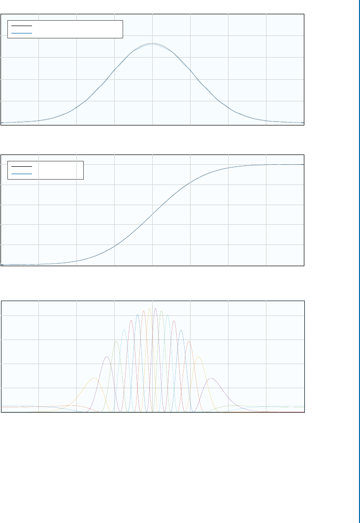
Figure 6.4: Top and middle: marginal density functions estimated using channel representations
and maximum entropy reconstruction, compared with the true marginal densities. Bottom: basis
functions for Copula estimation. e basis functions are regularly spaced on Œ0I1 and mapped
back to the original domain using the inverse estimated cumulative function. When estimating
the Copula, samples are instead mapped by the estimated cumulative function. Figure based
on Öäll and Felsberg [2017].
..................Content has been hidden....................
You can't read the all page of ebook, please click here login for view all page.