15

Deep Learning in Finance

In recent years, we have seen many spectacular successes achieved by means of deep learning techniques. Deep neural networks have been successfully applied to tasks in which traditional machine learning algorithms could not succeed—large-scale image classification, autonomous driving, and superhuman performance when playing traditional games such as Go or classic video games (from Super Mario to StarCraft II). Almost yearly, we can observe the introduction of a new type of network that achieves state-of-the-art (SOTA) results and breaks some kind of performance record.

With the constant improvement in commercially available Graphics Processing Units (GPUs), the emergence of freely available processing power involving CPUs/GPUs (Google Colab, Kaggle, and so on), and the rapid development of different frameworks, deep learning continues to gain more and more attention among researchers and practitioners who want to apply the techniques to their business cases.

In this chapter, we are going to show two possible use cases of deep learning in the financial domain—predicting credit card default (a classification task) and forecasting time series. Deep learning proves to deliver great results with sequential data such as speech, audio, and video. That is why it naturally fits into working with sequential data such as time series—both univariate and multivariate. Financial time series are known to be erratic and complex, hence the reason why it is such a challenge to model them. Deep learning approaches are especially apt for the task, as they make no assumptions about the distribution of the underlying data and can be quite robust to noise.

In this chapter, we present the following recipes:

• Exploring fastai’s Tabular Learner
• Exploring Google’s TabNet
• Time series forecasting with Amazon’s DeepAR
• Time series forecasting with NeuralProphet

Exploring fastai’s Tabular Learner

Deep learning is not often associated with tabular or structured data, as this kind of data comes with some possible questions:

• How should we represent features in a way that can be understood by the neural networks? In tabular data, we often deal with numerical and categorical features, so we need to correctly represent both types of inputs.
• How do we use feature interactions, both between the features themselves and the target?
• How do we effectively sample the data? Tabular datasets tend to be smaller than typical datasets used for solving computer vision or NLP problems. There is no easy way to apply augmentation, such as random cropping or rotation in the case of images. Also, there is no general large dataset with some universal properties, based on which we could easily apply transfer learning.
• How do we interpret the predictions of a neural network?

That is why practitioners tend to use traditional machine learning approaches (often based on some kind of gradient-boosted trees) to approach tasks involving structured data. However, a potential benefit of using deep learning for structured data is the fact that it requires much less feature engineering and domain knowledge.

In this recipe, we present how to successfully use deep learning for tabular data. To do so, we use the popular fastai library, which is built on top of PyTorch.

Some of the benefits of working with the fastai library are:

• It provides a selection of APIs that greatly simplify working with Artificial Neural Networks (ANNs)—from loading and batching the data to training the model
• It incorporates a selection of empirically tested best approaches to using deep learning for various tasks, such as image classification, NLP, and tabular data (both classification and regression problems)
• It handles the data preprocessing automatically—we just need to define which operations we want to apply

What makes fastai stand out is the use of entity embedding (or embedding layers) for categorical data. By using it, the model can learn some potentially meaningful relationships between the observations of categorical features. You can think of embeddings as latent features. For each categorical column, there is a trainable embedding matrix and each unique value has a designated vector mapped to it. Thankfully, fastai does all of that for us.

Using entity embedding comes with quite a few advantages. First, it reduces memory usage and speeds up the training of neural networks as compared to using one-hot encoding. Second, it maps similar values close to each other in the embedding space, which reveals the intrinsic properties of the categorical variables. Third, the technique is especially useful for datasets with many high-cardinality features, when other approaches tend to result in overfitting.

In this recipe, we apply deep learning to a classification problem based on the credit card default dataset. We have already used this dataset in Chapter 13, Applied Machine Learning: Identifying Credit Default.

How to do it…

Execute the following steps to train a neural network to classify defaulting customers:

1. Import the libraries:

   from fastai.tabular.all import *
   from sklearn.model_selection import train_test_split
   from chapter_15_utils import performance_evaluation_report_fastai
   import pandas as pd
   
2. Load the dataset from a CSV file:

   df = pd.read_csv("../Datasets/credit_card_default.csv",
                    na_values="")
   
3. Define the target, lists of categorical/numerical features, and preprocessing steps:

   TARGET = "default_payment_next_month"
   cat_features = list(df.select_dtypes("object").columns)
   num_features = list(df.select_dtypes("number").columns)
   num_features.remove(TARGET)
   preprocessing = [FillMissing, Categorify, Normalize]
   
4. Define the splitter used to create training and validation sets:

   splits = RandomSplitter(valid_pct=0.2, seed=42)(range_of(df))
   splits
   

   Executing the snippet generates the following previews of the datasets:

   ((#24000) [27362,16258,19716,9066,1258,23042,18939,24443,4328,4976...],
    (#6000) [7542,10109,19114,5209,9270,15555,12970,10207,13694,1745...])
   

5. Create the TabularPandas dataset:

   tabular_df = TabularPandas(
       df,
       procs=preprocessing,
       cat_names=cat_features,
       cont_names=num_features,
       y_names=TARGET,
       y_block=CategoryBlock(),
       splits=splits
   )
   PREVIEW_COLS = ["sex", "education", "marriage",
                   "payment_status_sep", "age_na", "limit_bal",
                   "age", "bill_statement_sep"]
   tabular_df.xs.iloc[:5][PREVIEW_COLS]
   

   Executing the snippet generates the following preview of the dataset:

   

   Figure 15.1: The preview of the encoded dataset

   We printed only a small selection of columns to keep the DataFrame readable. We can observe the following:

   • The categorical columns are encoded using a label encoder
   • The continuous columns are normalized
   • The continuous column that had missing values (age) has an extra column with an encoding indicating whether the particular value was missing before imputation

6. Define a DataLoaders object from the TabularPandas dataset:

   data_loader = tabular_df.dataloaders(bs=64, drop_last=True)
   data_loader.show_batch()
   

   Executing the snippet generates the following preview of the batch:

   

   Figure 15.2: The preview of a batch from the DataLoaders object

   As we can see in Figure 15.2, the features here are in their original representation.

7. Define the metrics of choice and the tabular learner:

   recall = Recall()
   precision = Precision()
   learn = tabular_learner(
       data_loader,
       [500, 200],
       metrics=[accuracy, recall, precision]
   )
   learn.model
   

   Executing the snippet prints the schema of the model:

   TabularModel(
     (embeds): ModuleList(
       (0): Embedding(3, 3)
       (1): Embedding(5, 4)
       (2): Embedding(4, 3)
       (3): Embedding(11, 6)
       (4): Embedding(11, 6)
       (5): Embedding(11, 6)
       (6): Embedding(11, 6)
       (7): Embedding(10, 6)
       (8): Embedding(10, 6)
       (9): Embedding(3, 3)
     )
     (emb_drop): Dropout(p=0.0, inplace=False)
     (bn_cont): BatchNorm1d(14, eps=1e-05, momentum=0.1, affine=True, track_running_stats=True)
     (layers): Sequential(
       (0): LinBnDrop(
         (0): Linear(in_features=63, out_features=500, bias=False)
         (1): ReLU(inplace=True)
         (2): BatchNorm1d(500, eps=1e-05, momentum=0.1, affine=True, track_running_stats=True)
       )
       (1): LinBnDrop(
         (0): Linear(in_features=500, out_features=200, bias=False)
         (1): ReLU(inplace=True)
         (2): BatchNorm1d(200, eps=1e-05, momentum=0.1, affine=True, track_running_stats=True)
       )
       (2): LinBnDrop(
         (0): Linear(in_features=200, out_features=2, bias=True)
       )
     )
   )
   

   To provide an interpretation of the embeddings, Embedding(11, 6) means that a categorical embedding was created with 11 input values and 6 output latent features.

8. Find the suggested learning rate:

   learn.lr_find()
   

   Executing the snippet generates the following plot:

   

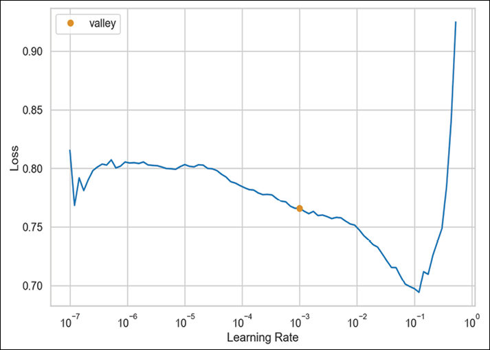
   Figure 15.3: The suggested learning rate for our model

   It also prints the following output with the exact value of the suggested learning rate:

   SuggestedLRs(valley=0.0010000000474974513)
   

9. Train the tabular learner:

   learn.fit(n_epoch=25, lr=1e-3, wd=0.2)
   

   While the model is training, we can observe the updates of its performance after each epoch. We present a snippet below.

   

   Figure 15.4: The first 10 epochs of the Tabular learner’s training

   In the first 10 epochs, the losses are still a bit erratic and increase/decrease over time. The same goes for the evaluation metrics.

10. Plot the losses:

    learn.recorder.plot_loss()
    

    Executing the snippet generates the following plot:

    

    Figure 15.5: The training and validation loss over training time (batches)

    We can observe that the validation loss plateaued a bit, with some bumps every now and then. It might mean that the model is a bit too complex for our data and we might want to reduce the size of the hidden layers.

11. Define the validation DataLoaders:

    valid_data_loader = learn.dls.test_dl(df.loc[list(splits[1])])
    
12. Evaluate the performance on the validation set:

    learn.validate(dl=valid_data_loader)
    

    Executing the snippet generates the following output:

    (#4)[0.424113571643829,0.8248333334922,0.36228482003129,0.66237482117310]
    

    These are the metrics for the validation set: loss, accuracy, recall, and precision.

13. Get predictions for the validation set:

    preds, y_true = learn.get_preds(dl=valid_data_loader)
    

    y_true contains the actual labels from the validation set. The preds object is a tensor containing the predicted probabilities. It looks as follows:

    tensor([[0.8092, 0.1908],
            [0.9339, 0.0661],
            [0.8631, 0.1369],
            ...,
            [0.9249, 0.0751],
            [0.8556, 0.1444],
            [0.8670, 0.1330]])
    

    To get the predicted classes from it, we can use the following command:

    preds.argmax(dim=-1)
    

14. Inspect the performance evaluation metrics:

    perf = performance_evaluation_report_fastai(
        learn, valid_data_loader, show_plot=True
    )
    

    Executing the snippet generates the following plot:

Figure 15.6: The performance evaluation of the Tabular learner’s prediction of the validation set

The perf object is a dictionary containing various evaluation metrics. We have not presented it here for brevity, but we can also see that accuracy, precision, and recall have the same values as we saw in Step 12.

How it works…

In Step 2, we loaded the dataset into Python using the read_csv function. While doing so, we indicated which symbol represents the missing values.

In Step 3, we identified the dependent variable (the target), as well as both numerical and categorical features. To do so, we used the select_dtypes methods and indicated which data type we wanted to extract. We stored the features in lists. We also had to remove the dependent variable from the list containing the numerical features. Lastly, we created a list containing all the transformations we wanted to apply to the data. We selected the following:

• FillMissing: Missing values will be filled depending on the data type. In the case of categorical variables, missing values become a separate category. In the case of continuous features, the missing values are filled using the median of the feature’s values (default approach), the mode, or with a constant value. Additionally, an extra column is added with a flag whether the value was missing or not.
• Categorify: Maps categorical features into their integer representation.
• Normalize: Features’ values are transformed such that they have zero mean and unit variance. This makes training neural networks easier.

It is important to note that the same transformations will be applied to both the training and validation sets. To prevent data leakage, the transformations are based solely on the training set.

In Step 4, we defined a split used for creating the training and validation sets. We used the RandomSplitter class, which does a stratified split under the hood. We indicated we wanted to split the data using the 80-20 ratio. Additionally, after instantiating the splitter, we also had to use the range_of function, which returns a list containing all the indices of our DataFrame.

In Step 5, we created a TabularPandas dataset. It is a wrapper around a pandas DataFrame, which adds a few convenient utilities on top—it handles all the preprocessing and splitting. While instantiating the TabularPandas class, we provided the original DataFrame, a list containing all the preprocessing steps, the names of the target and the categorical/continuous features, and the splitter object we defined in Step 4. We also specified y_block=CategoryBlock(). We have to do so when we are working with a classification problem and the target was already encoded into a binary representation (a column of zeroes and ones). Otherwise, it might be confused with a regression problem.

We can easily convert a TabularPandas object into a regular pandas DataFrame. We can use the xs method to extract the features and the ys method to extract the target. Additionally, we can use the cats and conts methods to extract categorical and continuous features, respectively. If we use any of the four methods directly on the TabularPandas object, we will extract the entire dataset. Alternatively, we can use the train and valid accessors to extract only one of the sets. For example, to extract the validation set features from a TabularPandas object called tabular_df, we could use the following snippet:

tabular_df.valid.xs

In Step 6, we converted the TabularPandas object into a DataLoaders object. To do so, we used the dataloaders method of the TabularPandas dataset. Additionally, we specified a batch size of 64 and that we wanted to drop the last incomplete batch. We displayed a sample batch using the show_batch method.

In Step 7, we defined the learner using tabular_learner. First, we instantiated additional metrics: precision and recall. When using fastai, metrics are expressed as classes (the name is spelled in uppercase) and we first need to instantiate them before passing them to the learner.

Then, we instantiated the learner. This is the place where we defined the network’s architecture. We decided to use a network with two hidden layers, with 500 and 200 neurons, respectively. Choosing the network’s architecture can often be considered more an art than science and may require a significant amount of trial and error. Another popular approach is to use an architecture that worked before for someone else, for example, based on academic papers, Kaggle competitions, blog articles, and so on. As for the metrics, we wanted to consider accuracy and the previously mentioned precision and recall.

As in the case of machine learning, it is crucial to prevent overfitting with neural networks. We want the networks to be able to generalize to new data. Some of the popular techniques used for tackling overfitting include the following:

• Weight decay: Each time the weights are updated, they are multiplied by a factor smaller than 1 (a rule of thumb is to use values between 0.01 and 0.1).
• Dropout: While training the NN, some activations are randomly dropped for each mini-batch. Dropout can also be used for the concatenated vector of embeddings of categorical features.
• Batch normalization: This technique reduces overfitting by making sure that a small number of outlying inputs does have too much impact on the trained network.

Then, we inspected the model’s architecture. In the output, we first saw the categorical embeddings and the corresponding dropout, or in this case, the lack of it. Then, in the (layers) section, we saw the input layer (63 input and 500 output features), followed by the ReLU (Rectified Linear Unit) activation function, and batch normalization. Potential dropout is governed in the LinBnDrop layer. The same steps were repeated for the second hidden layer and then the last linear layer produced the class probabilities.

In Step 8, we tried to determine the “good” learning rate. fastai provides a helper method, lr_find, which facilitates the process. It begins to train the network while increasing the learning rate—it starts with a very low one and increases to a very large one. Then, it plots the losses against the learning rates and displays the suggested value. We should aim for a value that is before the minimum value, but where the loss still improves (decreases).

In Step 9, we trained the neural network using the fit method of the learner. We’ll briefly describe the training algorithm. The entire training set is divided into batches. For each batch, the network is used to make predictions, which are compared to the target values and used to calculate the error. Then, the error is used to update the weights in the network. An epoch is a complete run through all the batches, in other words, using the entire dataset for training. In our case, we trained the network for 25 epochs. We additionally specified the learning rate and weight decay. In Step 10, we plotted the training and validation loss over batches.

In Step 11, we defined a validation dataloader. To identify the indices of the validation set, we extracted them from the splitter. In the next step, we evaluated the performance of the neural network on the validation set using the validate method of the learner object. As input for the method, we passed the validation dataloader.

In Step 13, we used the get_preds method to obtain the validation set predictions. To obtain the predictions from the preds object, we had to use the argmax method.

Lastly, we used the slightly modified helper function (used in the previous chapters) to recover evaluation metrics such as precision and recall.

There’s more…

Some noteworthy features of fastai for tabular datasets include:

• Using callbacks while training neural networks. Callbacks are used to insert some custom code/logic into the training loop at different times, for example, at the beginning of the epoch or at the beginning of the fitting process.
• fastai provides a helper function, add_datepart, which extracts a variety of features from columns containing dates (such as the purchase date). Some of the extracted features may include the day of the week, the day of the month, and a Boolean for the start/end of the month/quarter/year.
• We can use the predict method of a fitted tabular learner to predict the class directly for a single row of the source DataFrame.
• Instead of the fit method, we can also use the fit_one_cycle method. This employs the super-convergence policy. The underlying idea is to train the network with a varying learning rate. It starts at low values, increases to the specified maximum, and goes back to low values again. This approach is considered to work better than choosing a single learning rate.
• As we were working with a relatively small dataset and a simple model, we could have quite easily trained the NN on a CPU. fastai naturally supports using GPUs. For more information on how to use a GPU, please see fastai's documentation.
• Using custom indices for training and validation sets. This feature comes in handy when we are, for example, dealing with class imbalance and want to make sure that both the training and validation sets contain a similar ratio of classes. We can use IndexSplitter in combination with scikit-learn's StratifiedKFold. We show an example of the implementation in the following snippet:

  from sklearn.model_selection import StratifiedKFold
  X = df.copy()
  y = X.pop(TARGET)
  strat_split = StratifiedKFold(
      n_splits=5, shuffle=True, random_state=42
  )
  train_ind, test_ind = next(strat_split.split(X, y))
  ind_splits = IndexSplitter(valid_idx=list(test_ind))(range_of(df))
  tabular_df = TabularPandas(
      df,
      procs=preprocessing,
      cat_names=cat_features,
      cont_names=num_features,
      y_names=TARGET,
      y_block=CategoryBlock(),
      splits=ind_splits
  )
  

See also

For more information about fastai, we recommend the following:

• The fastai course website: https://course.fast.ai/.
• Howard, J., & Gugger, S. 2020. Deep Learning for Coders with fastai and PyTorch. O’Reilly Media. https://github.com/fastai/fastbook.

Additional resources are available here:

• Guo, C., & Berkhahn, F. 2016. Entity Embeddings of Categorical Variables. arXiv preprint arXiv:1604.06737.
• Ioffe, S., & Szegedy, C. 2015. Batch Normalization: Accelerating Deep Network Training by Reducing Internal Covariate Shift. arXiv preprint arXiv:1502.03167.
• Krogh, A., & Hertz, J. A. 1991. “A simple weight decay can improve generalization.” In Advances in neural information processing systems: 9950-957.
• Ryan, M. 2020. Deep Learning with Structured Data. Simon and Schuster.
• Shwartz-Ziv, R., & Armon, A. 2022. “Tabular data: Deep learning is not all you need”, Information Fusion, 81: 84-90.
• Smith, L. N. 2018. A disciplined approach to neural network hyperparameters: Part 1 – learning rate, batch size, momentum, and weight decay. arXiv preprint arXiv:1803.09820.
• Smith, L. N., & Topin, N. 2019, May. Super-convergence: Very fast training of neural networks using large learning rates. In Artificial intelligence and machine learning for multi-domain operations applications (1100612). International Society for Optics and Photonics.
• Srivastava, N., Hinton, G., Krizhevsky, A., Sutskever, I., & Salakhutdinov, R. 2014. “Dropout: a simple way to prevent neural networks from overfitting”, The Journal of Machine Learning Research, 15(1): 1929-1958.

Exploring Google’s TabNet

Another possible approach to modeling tabular data using neural networks is Google’s TabNet. As TabNet is a complex model, we will not describe its architecture in depth. For that, we refer you to the original paper (mentioned in the See also section). Instead, we provide a high-level overview of TabNet’s main features:

• TabNet uses raw tabular data without any preprocessing.
• The optimization procedure used in TabNet is based on gradient descent.
• TabNet combines the ability of neural networks to fit very complex functions and the feature selection properties of tree-based algorithms. By using sequential attention to choose features at each decision step, TabNet can focus on learning from only the most useful features.
• TabNet’s architecture employs two critical building blocks: a feature transformer and an attentive transformer. The former processes the features into a more useful representation. The latter selects the most relevant features to process during the next step.
• TabNet also has another interesting component—a learnable mask of the input features. The mask should be sparse, that is, it should select a small set of features to solve the prediction task. In contrast to decision trees (and other tree-based models), the feature selection enabled by the mask allows for soft decisions. In practice, it means that a decision can be made on a larger range of values instead of a single threshold value.
• TabNet’s feature selection is instance-wise, that is, different features can be selected for each observation (row) in the training data.
• TabNet is also quite unique as it uses a single deep learning architecture for both feature selection and reasoning.
• In contrast to the vast majority of deep learning models, TabNet is interpretable (to some extent). All of the design choices allow TabNet to offer both local and global interpretability. The local interpretability allows us to visualize the feature importances and how they are combined for a single row. The global one provides an aggregate measure of each feature’s contribution to the trained model (over the entire dataset).

In this recipe, we show how to apply TabNet (its PyTorch implementation) to the same credit card default dataset we covered in the previous example.

How to do it…

Execute the following steps to train a TabNet classifier using the credit card fraud dataset:

1. Import the libraries:

   from sklearn.model_selection import train_test_split
   from sklearn.preprocessing import LabelEncoder
   from sklearn.metrics import recall_score
   from pytorch_tabnet.tab_model import TabNetClassifier
   from pytorch_tabnet.metrics import Metric
   import torch
   import pandas as pd
   import numpy as np
   
2. Load the dataset from a CSV file:

   df = pd.read_csv("../Datasets/credit_card_default.csv",
                    na_values="")
   
3. Separate the target from the features and create lists with numerical/categorical features:

   X = df.copy()
   y = X.pop("default_payment_next_month")
   cat_features = list(X.select_dtypes("object").columns)
   num_features = list(X.select_dtypes("number").columns)
   
4. Impute missing values in the categorical features, encode them using LabelEncoder, and store the number of unique categories per feature:

   cat_dims = {}
   for col in cat_features:
       label_encoder = LabelEncoder()
       X[col] = X[col].fillna("Missing")
       X[col] = label_encoder.fit_transform(X[col].values)
       cat_dims[col] = len(label_encoder.classes_)
   cat_dims
   

   Executing the snippet generates the following output:

   {'sex': 3,
    'education': 5,
    'marriage': 4,
    'payment_status_sep': 10,
    'payment_status_aug': 10,
    'payment_status_jul': 10,
    'payment_status_jun': 10,
    'payment_status_may': 9,
    'payment_status_apr': 9}
   

   Based on the EDA, we would assume that the sex feature takes two unique values. However, as we have imputed the missing values with the Missing category, there are three unique possibilities.

5. Create a train/valid/test split using the 70-15-15 split:

   # create the initial split - training and temp
   X_train, X_temp, y_train, y_temp = train_test_split(
       X, y,
       test_size=0.3,
       stratify=y,
       random_state=42
   )
   # create the valid and test sets
   X_valid, X_test, y_valid, y_test = train_test_split(
       X_temp, y_temp,
       test_size=0.5,
       stratify=y_temp,
       random_state=42
   )
   
6. Impute the missing values in the numerical features across all the sets:

   for col in num_features:
       imp_mean = X_train[col].mean()
       X_train[col] = X_train[col].fillna(imp_mean)
       X_valid[col] = X_valid[col].fillna(imp_mean)
       X_test[col] = X_test[col].fillna(imp_mean)
   
7. Prepare lists with the indices of categorical features and the number of unique categories:

   features = X.columns.to_list()
   cat_ind = [features.index(feat) for feat in cat_features]
   cat_dims = list(cat_dims.values())
   
8. Define a custom recall metric:

   class Recall(Metric):
       def __init__(self):
           self._name = "recall"
           self._maximize = True
       def __call__(self, y_true, y_score):
           y_pred = np.argmax(y_score, axis=1)
           return recall_score(y_true, y_pred)
   
9. Define TabNet’s parameters and instantiate the classifier:

   tabnet_params = {
       "cat_idxs": cat_ind,
       "cat_dims": cat_dims,
       "optimizer_fn": torch.optim.Adam,
       "optimizer_params": dict(lr=2e-2),
       "scheduler_params": {
           "step_size":20,
           "gamma":0.9
       },
       "scheduler_fn": torch.optim.lr_scheduler.StepLR,
       "mask_type": "sparsemax",
       "seed": 42,
   }
   tabnet = TabNetClassifier(**tabnet_params)
   
10. Train the TabNet classifier:

    tabnet.fit(
        X_train=X_train.values,
        y_train=y_train.values,
        eval_set=[
            (X_train.values, y_train.values),
            (X_valid.values, y_valid.values)
        ],
        eval_name=["train", "valid"],
        eval_metric=["auc", Recall],
        max_epochs=200,
        patience=20,
        batch_size=1024,
        virtual_batch_size=128,
        weights=1,
    )
    

    Below we can see an abbreviated log from the training procedure:

    epoch 0  | loss: 0.69867 | train_auc: 0.61461 | train_recall: 0.3789  | valid_auc: 0.62232 | valid_recall: 0.37286 |  0:00:01s
    epoch 1  | loss: 0.62342 | train_auc: 0.70538 | train_recall: 0.51539 | valid_auc: 0.69053 | valid_recall: 0.48744 |  0:00:02s
    epoch 2  | loss: 0.59902 | train_auc: 0.71777 | train_recall: 0.51625 | valid_auc: 0.71667 | valid_recall: 0.48643 |  0:00:03s
    epoch 3  | loss: 0.59629 | train_auc: 0.73428 | train_recall: 0.5268  | valid_auc: 0.72767 | valid_recall: 0.49447 |  0:00:04s
    …
    epoch 42 | loss: 0.56028 | train_auc: 0.78509 | train_recall: 0.6028  | valid_auc: 0.76955 | valid_recall: 0.58191 |  0:00:47s
    epoch 43 | loss: 0.56235 | train_auc: 0.7891  | train_recall: 0.55651 | valid_auc: 0.77126 | valid_recall: 0.5407  |  0:00:48s
    Early stopping occurred at epoch 43 with best_epoch = 23 and best_valid_recall = 0.6191
    Best weights from best epoch are automatically used!
    

11. Prepare the history DataFrame and plot the scores over epochs:

    history_df = pd.DataFrame(tabnet.history.history)
    

    Then, we start by plotting the loss over epochs:

    history_df["loss"].plot(title="Loss over epochs")
    

    Executing the snippet generates the following plot:

    

    Figure 15.7: Training loss over epochs

    Then, in a similar manner, we generated a plot showing the recall score over the epochs. For brevity, we have not included the code generating the plot.

    

    Figure 15.8: Training and validation recall over epochs

12. Create predictions for the test set and evaluate their performance:

    y_pred = tabnet.predict(X_test.values)
    print(f"Best validation score: {tabnet.best_cost:.4f}")
    print(f"Test set score: {recall_score(y_test, y_pred):.4f}")
    

    Executing the snippet generates the following output:

    Best validation score: 0.6191
    Test set score: 0.6275
    

    As we can see, the test set performance is slightly better than the recall score calculated using the validation set.

13. Extract and plot the global feature importance:

    tabnet_feat_imp = pd.Series(tabnet.feature_importances_,
                                index=X_train.columns)
    (
        tabnet_feat_imp
        .nlargest(20)
        .sort_values()
        .plot(kind="barh",
              title="TabNet's feature importances")
    )
    

    Executing the snippet generates the following plot:

Figure 15.9: Global feature importance values extracted from the fitted TabNet classifier

According to TabNet, the most important features for predicting defaults in October were the payment statuses in September, July, and May. Another important feature was the limit balance.

Two things are worth mentioning at this point. First, the most important features are similar to the ones we identified in the Investigating feature importance recipe in Chapter 14, Advanced Concepts for Machine Learning Projects. Second, the feature importance is on a feature level, not on a feature and category level, as we could have seen while using one-hot encoding on categorical features.

How it works…

After importing the libraries, we loaded the dataset from a CSV file. Then, we separated the target from the features and extracted the names of the categorical and numerical features. We stored those as lists.

In Step 4, we carried out a few operations on the categorical features. First, we imputed any missing values with a new category—Missing. Then, we used scikit-learn's LabelEncoder to encode each of the categorical columns. While doing so, we populated a dictionary containing the number of unique categories (including the newly created one for the missing values) for each of the categorical features.

In Step 5, we created a training/validation/test split using the train_test_split function. We decided to use the 70-15-15 split for the sets. As the dataset is imbalanced (the minority class is observable in approximately 22% of observations), we used stratification while splitting the data.

In Step 6, we imputed the missing values for the numerical features. We filled in the missing values using the average value calculated over the training set.

In Step 7, we prepared two lists. The first one contained the numerical indices of the categorical features, while the second one contained the number of unique categories per categorical feature. It is crucial that the lists are aligned so that the indices of the features correspond to those features’ number of unique categories.

In Step 8, we created a custom recall metric. pytorch-tabnet offers a few metrics (for classification problems, those include accuracy, ROC AUC, and balanced accuracy), but we can easily define more. To create the custom metric, we did the following:

• We defined a class inheriting from the Metric class.
• In the __init__ method, we defined the name of the metric (as visible in the training logs) and indicated whether the goal is to maximize the metric. That is the case for recall.
• In the __call__ method, we calculated the value of recall using the recall_score function from scikit-learn. But first, we had to convert the array containing the predicted probabilities of each class into an object containing the predicted class. We did so using the np.argmax function.

In Step 9, we defined some of the hyperparameters of TabNet and instantiated the model. pytorch-tabnet offers a familiar scikit-learn API to train TabNet for either a classification or regression task. This way, we do not have to be familiar with PyTorch to train the model. First, we defined a dictionary containing the hyperparameters of the model.

In general, some of the hyperparameters are defined on the model level (passed to the class while instantiating it), while the other ones are defined on the fit level (passed to the model while using the fit method). At this point, we defined the model hyperparameters:

• The indices of the categorical features and the corresponding numbers of unique classes
• ADAM as the selected optimizer
• The learning rate scheduler
• The type of masking
• Random seed

Among all of those, the learning rate scheduler might require a bit of clarification. As per TabNet’s documentation, we used a stepwise decay for the learning rate. To do so, we specified torch.optim.lr_scheduler.StepLR as the scheduler function. Then, we provided a few more parameters. Initially, we set the learning rate to 0.02 in the optimizer_params. Then, we defined the stepwise decay parameters in scheduler_params. We specified that after every 20 epochs, we wanted to apply the decay rate of 0.9. In practice, it means that after 20 epochs, the learning rate will be 0.9 times 0.02, which is equal to 0.018. The decay then continues after every 20 epochs.

Having done so, we instantiated the TabNetClassifier class using the specified hyperparameters. By default, TabNet uses a cross-entropy loss function for classification problems and the MSE for regression tasks.

In Step 10, we trained TabNetClassifier using its fit method. We provided quite a few parameters:

• Training data
• Evaluation sets—in this case, we used both the training and validation sets so that after each epoch we see the metrics calculated over both sets
• The names of the evaluation sets
• The metrics to be used for evaluation—we used the ROC AUC and the custom recall metric defined in Step 8
• The maximum number of epochs
• The patience parameter, which states that if we do not observe an improvement in the evaluation metrics over X consecutive epochs, the training will stop and we will use the weights from the best epoch for predictions
• The batch size and the virtual batch size (used for ghost batch normalization; please see the There’s more... section for more details)
• The weights parameter, which is only available for classification problems. It corresponds to sampling, which can be of great help when dealing with class imbalance. Setting it to 0 results in no sampling. Setting it to 1 turns on the sampling with the weights proportional to the inverse class occurrences. Lastly, we can provide a dictionary with custom weights for the classes.

One thing to note about TabNet’s training is that the dataset we provide must be numpy arrays instead of pandas DataFrames. That is why we used the values method to extract the arrays from the DataFrames. The need to use numpy arrays is also the reason why we had to define the numeric indices of the categorical features, instead of providing a list with feature names.

In Step 11, we extracted the training information from the history attribute of the fitted TabNet model. It contains the same information that was visible in the training log, that is, the loss, learning rate, and evaluation metrics over epochs. Then, we plotted the loss and recall over epochs.

In Step 12, we created the predictions using the predict method. Similar to the training step, we also had to provide the input features as a numpy array. As in scikit-learn, the predict method returns the predicted class, while we could use the predict_proba method to get the class probabilities. We also calculated the recall score over the test set using the recall_score function from scikit-learn.

In the last step, we extracted the global feature importance values. Similar to scikit-learn models, they are stored under the feature_importances_ attribute of a fitted model. Then, we plotted the 20 most important features. It is worth mentioning that the global feature importance values are normalized and they sum up to 1.

There’s more…

Here are a few more interesting points about TabNet and its implementation in PyTorch:

• TabNet uses ghost batch normalization to train large batches of data and provide better generalization at the same time. The idea behind the procedure is that we split the input batch into equal-sized sub-batches (determined by the virtual batch size parameter). Then, we apply the same batch normalization layer to those sub-batches.
• pytorch-tabnet allows us to apply custom data augmentation pipelines during training. Currently, the library offers using SMOTE for both classification and regression tasks.
• TabNet can be pre-trained as an unsupervised model, which can then lead to improved performance. While pre-training, certain cells are deliberately masked and the model learns the relationships between these censored cells and the adjacent columns by predicting the missing (masked) values. We can then use those weights for a supervised task. By learning about the relationships between features, the unsupervised representation learning acts as an improved encoder model for the supervised learning task. When pre-training, we can decide what percentage of features is masked.
• TabNet uses sparsemax as the masking function. In general, sparsemax is a non-linear normalization function with a sparser distribution than the popular softmax function. This function allows the neural network to more effectively select the important features. Additionally, the function employs sparsity regularization (its strength is determined by a hyperparameter) to penalize less sparse masks. The pytorch-tabnet library also contains the EntMax masking function.
• In the recipe, we have presented how to extract global feature importance. To extract the local ones, we can use the explain method of a fitted TabNet model. It returns two elements: a matrix containing the importance of each observation and feature, and the attention masks used by the model for feature selection.

See also

• Arik, S. Ö., & Pfister, T. 2021, May. Tabnet: Attentive interpretable tabular learning. In Proceedings of the AAAI Conference on Artificial Intelligence, 35(8): 6679-6687.
• The original repository containing TabNet’s implementation described in the abovementioned paper: https://github.com/google-research/google-research/tree/master/tabnet.

Time series forecasting with Amazon’s DeepAR

We have already covered time series analysis and forecasting in Chapter 6, Time Series Analysis and Forecasting, and Chapter 7, Machine Learning-Based Approaches to Time Series Forecasting. This time, we will have a look at an example of a deep learning approach to time series forecasting. In this recipe, we cover Amazon’s DeepAR model. The model was originally developed as a tool for demand/sales forecasting at the scale of hundreds if not thousands of stock-keeping units (SKUs).

The architecture of DeepAR is beyond the scope of this book. Hence, we will only focus on some of the key characteristics of the model. Those are listed below:

• DeepAR creates a global model used for all the considered time series. It implements LSTM cells in an architecture that allows for training using hundreds or thousands of time series simultaneously. The model also uses an encoder-decoder setup, which is common in sequence-to-sequence models.
• DeepAR allows for using a set of covariates (external regressors) related to the target time series.
• The model requires minimal feature engineering. It automatically creates relevant time series features (depending on the granularity of the data, this might be the day of the month, day of the year, and so on) and it learns seasonal patterns from the provided covariates across time series.
• DeepAR offers probability forecasts based on Monte Carlo sampling—it calculates consistent quantile estimates.
• The model is able to create forecasts for time series with little historical data by learning from similar time series. This is a potential solution to the cold start problem.
• The model can use various likelihood functions.

In this recipe, we will train a DeepAR model using around 100 time series of daily stock prices from the years 2020 and 2021. Then, we will create 20-day-ahead forecasts covering the last 20 business days of 2021.

Before moving forward, we wanted to highlight that we are using time series of stock prices just for illustratory purposes. Deep learning models excel when trained on hundreds if not thousands of time series. We have selected stock prices as those are the easiest to download. As we have already mentioned, accurately forecasting stock prices, especially with a long forecast horizon, is very difficult if not simply impossible.

How to do it…

Execute the following steps to train the DeepAR model using stock prices as the input time series:

1. Import the libraries:

   import pandas as pd
   import torch
   import yfinance as yf
   from random import sample, seed
   import pytorch_lightning as pl
   from pytorch_lightning.callbacks import EarlyStopping
   from pytorch_forecasting import DeepAR, TimeSeriesDataSet
   
2. Download the tickers of the S&P 500 constituents and sample 100 random tickers from the list:

   df = pd.read_html(
       "https://en.wikipedia.org/wiki/List_of_S%26P_500_companies"
   )
   df = df[0]
   seed(44)
   sampled_tickers = sample(df["Symbol"].to_list(), 100)
   
3. Download the historical stock prices of the selected stocks:

   raw_df = yf.download(sampled_tickers,
                        start="2020-01-01",
                        end="2021-12-31")
   
4. Keep the adjusted close price and remove the stocks with missing values:

   df = raw_df["Adj Close"]
   df = df.loc[:, ~df.isna().any()]
   selected_tickers = df.columns
   

   After removing the stocks that have at least one missing value in the period of interest, we are left with 98 stocks.

5. Convert the data’s format from wide to long and add the time index:

   df = df.reset_index(drop=False) 
    
   df = ( 
       pd.melt(df, 
               id_vars=["Date"], 
               value_vars=selected_tickers, 
               value_name="price"
       ).rename(columns={"variable": "ticker"}) 
   )
   df["time_idx"] = df.groupby("ticker").cumcount() 
   df
   

   Executing the snippet generates the following preview of the DataFrame:

   

   Figure 15.10: The preview of the input DataFrame for the DeepAR model

6. Define constants used for setting up the model’s training:

   MAX_ENCODER_LENGTH = 40
   MAX_PRED_LENGTH = 20
   BATCH_SIZE = 128
   MAX_EPOCHS = 30
   training_cutoff = df["time_idx"].max() - MAX_PRED_LENGTH
   
7. Define the training and validation datasets:

   train_set = TimeSeriesDataSet(
       df[lambda x: x["time_idx"] <= training_cutoff],
       time_idx="time_idx",
       target="price",
       group_ids=["ticker"],
       time_varying_unknown_reals=["price"],
       max_encoder_length=MAX_ENCODER_LENGTH,
       max_prediction_length=MAX_PRED_LENGTH,
   )
   valid_set = TimeSeriesDataSet.from_dataset(
       train_set, df, min_prediction_idx=training_cutoff+1
   )
   
8. Get the dataloaders from the datasets:

   train_dataloader = train_set.to_dataloader(
       train=True, batch_size=BATCH_SIZE
   )
   valid_dataloader = valid_set.to_dataloader(
       train=False, batch_size=BATCH_SIZE
   )
   
9. Define the DeepAR model and find the suggested learning rate:

   pl.seed_everything(42)
   deep_ar = DeepAR.from_dataset(
       train_set,
       learning_rate=1e-2,
       hidden_size=30,
       rnn_layers=4
   )
   trainer = pl.Trainer(gradient_clip_val=1e-1)
   res = trainer.tuner.lr_find(
       deep_ar,
       train_dataloaders=train_dataloader,
       val_dataloaders=valid_dataloader,
       min_lr=1e-5,
       max_lr=1e0,
       early_stop_threshold=100,
   )
   fig = res.plot(show=True, suggest=True)
   

   Executing the snippet generates the following plot, in which the red dot indicates the suggested learning rate.

   

   Figure 15.11: The suggested learning rate for training the DeepAR model

10. Train the DeepAR model:

    pl.seed_everything(42)
    deep_ar.hparams.learning_rate = res.suggestion()
    early_stop_callback = EarlyStopping(
        monitor="val_loss",
        min_delta=1e-4,
        patience=10
    )
    trainer = pl.Trainer(
        max_epochs=MAX_EPOCHS,
        gradient_clip_val=0.1,
        callbacks=[early_stop_callback]
    )
    trainer.fit(
        deep_ar,
        train_dataloaders=train_dataloader,
        val_dataloaders=valid_dataloader,
    )
    
11. Extract the best DeepAR model from a checkpoint:

    best_model = DeepAR.load_from_checkpoint(
        trainer.checkpoint_callback.best_model_path
    )
    
12. Create the predictions for the validation set and plot 5 of them:

    raw_predictions, x = best_model.predict(
        valid_dataloader,
        mode="raw",
        return_x=True,
        n_samples=100
    )
    tickers = valid_set.x_to_index(x)["ticker"]
    for idx in range(5):
        best_model.plot_prediction(
            x, raw_predictions, idx=idx, add_loss_to_title=True
        )
        plt.suptitle(f"Ticker: {tickers.iloc[idx]}")
    

    In the snippet, we generated 100 predictions and plotted 5 of them for visual inspection. For brevity, we will only show two of them. But we highly encourage inspecting more plots to better understand the model’s performance.

Figure 15.12: DeepAR’s forecast for the ABMD stock

Figure 15.13: DeepAR’s forecast for the ADM stock

The plots show the forecast for two stocks for the last 20 business days of 2021, together with the corresponding quantile estimates. While the forecasts do not perform that well, we can see that at the very least the actual values are within the provided quantile estimates.

We will not spend more time evaluating the performance of the model and its forecasts, as the main idea was to present how the DeepAR model works and how to use it to generate the forecasts. However, we will mention a few potential improvements. First, we could have trained for more epochs, as we did not look into the model’s convergence. We have used early stopping, but it was not triggered while training. Second, we have used quite a few arbitrary values to define the network’s architecture. In a real-life scenario, we should use a hyperparameter optimization routine of our choice to identify the best values for our task at hand.

How it works…

In Step 1, we imported the required libraries. To use the DeepAR model, we decided to use the PyTorch Forecasting library. It is a library built on top of PyTorch Lightning and allows us to easily use state-of-the-art deep learning models for time series forecasting. The models can be trained using GPUs and we can also refer to TensorBoard for inspection of the training logs.

In Step 2, we downloaded the list containing the constituents of the S&P 500 index. Then, we randomly sampled 100 of those and stored the results in a list. We sampled the tickers to make the training faster. It would definitely be interesting, and beneficial to the model, to repeat the exercise with all of the stocks.

In Step 3, we downloaded the historical stock prices from the years 2020 and 2021 using the yfinance library. In the next step, we had to apply further preprocessing. We only kept the adjusted close prices and we removed the stocks with any missing values.

In Step 5, we continued with the preprocessing. We converted the DataFrame from a wide to a long format and then added the time index. The DeepAR implementation works with an integer time index instead of dates, hence we used the cumcount method combined with the groupby method to create the time index for each of the considered stocks.

In Step 6, we defined some of the constants used for the training procedure, for example, the max length of the encoder step, the number of observations we wanted to forecast into the future, the max number of training epochs, and so on. We also specified which time index cuts off the training from the validation.

In Step 7, we defined the training and validation datasets. We did so using the TimeSeriesDataSet class, the responsibilities of which include:

• The handling of variable transformations
• The treatment of missing values
• Storing information about static and time-varying variables (both known and unknown in the future)
• Randomized subsampling

While defining the training dataset, we had to provide the training data (filtered using the previously defined cutoff point), the name of the columns containing the time index, the target, group IDs (in our case, these were the tickers), the encoder length, and the forecast horizon.

In Step 8, we converted the datasets into dataloaders using the to_dataloader method of a TimeSeriesDataSet.

In Step 9, we defined the DeepAR model using the from_dataset method of the DeepAR class. This way, we did not have to repeat what we had already specified while creating the TimeSeriesDataSet objects. Additionally, we specified the learning rate, the size of the hidden layers, and the number of RNN layers. The latter two are the most important hyperparameters of the DeepAR model and they should be tuned using some HPO framework, for example, Hyperopt or Optuna. Then, we used PyTorch Lightning’s Trainer class to find the best learning rate for our model.

In Step 10, we trained the DeepAR model using the identified learning rate. Additionally, we specified the early stopping callback, which stops the training if there is no significant (defined by us) improvement in the validation loss over 10 epochs.

In Step 11, we extracted the best model from a checkpoint. Then, we used the best model to create predictions using the predict method. We created predictions for 100 sequences available in the validation dataloader. We indicated that we wanted to extract the raw predictions (this option returns a dictionary with the predictions and additional information such as the corresponding quantiles, and so on) and the inputs used for generating those predictions. Then, we plotted the predictions using the plot_prediction method of the fitted DeepAR model.

There’s more…

PyTorch Forecasting also allows us to easily train a DeepVAR model, which is the multivariate counterpart of DeepAR. Originally, Salinas et al. (2019) called this model VEC-LSTM.

In this section, we show how to adjust the code used for training the DeepAR model to train a DeepVAR model instead:

1. Import the libraries:

   from pytorch_forecasting.metrics import MultivariateNormalDistributionLoss
   import seaborn as sns
   import numpy as np
   
2. Define the dataloaders again:

   train_set = TimeSeriesDataSet(
       df[lambda x: x["time_idx"] <= training_cutoff],
       time_idx="time_idx",
       target="price",
       group_ids=["ticker"],
       static_categoricals=["ticker"],  
       time_varying_unknown_reals=["price"],
       max_encoder_length=MAX_ENCODER_LENGTH,
       max_prediction_length=MAX_PRED_LENGTH,
   )
   valid_set = TimeSeriesDataSet.from_dataset(
       train_set, df, min_prediction_idx=training_cutoff+1
   )
   train_dataloader = train_set.to_dataloader(
       train=True,
       batch_size=BATCH_SIZE,
       batch_sampler="synchronized"
   )
   valid_dataloader = valid_set.to_dataloader(
       train=False,
       batch_size=BATCH_SIZE,
       batch_sampler="synchronized"
   )
   

   There are two differences in this step. First, when we created the training dataset, we also specified the static_categoricals argument. Because we will forecast correlations, it is important to use series characteristics such as their tickers. Second, we also had to specify batch_sampler="synchronized" while creating the dataloaders. Using that option ensures that samples passed to the decoder are aligned in time.

3. Define the DeepVAR model and find the learning rate:

   pl.seed_everything(42)
   deep_var = DeepAR.from_dataset(
       train_set,
       learning_rate=1e-2,
       hidden_size=30,
       rnn_layers=4,
       loss=MultivariateNormalDistributionLoss()
   )
   trainer = pl.Trainer(gradient_clip_val=1e-1)
   res = trainer.tuner.lr_find(
       deep_var,
       train_dataloaders=train_dataloader,
       val_dataloaders=valid_dataloader,
       min_lr=1e-5,
       max_lr=1e0,
       early_stop_threshold=100,
   )
   

   The last difference between training DeepVAR and DeepAR models is that for the former, we use MultivariateNormalDistributionLoss as the loss, instead of the default NormalDistributionLoss.

4. Train the DeepVAR model using the selected learning rate:

   pl.seed_everything(42)
   deep_var.hparams.learning_rate = res.suggestion()
   early_stop_callback = EarlyStopping(
       monitor="val_loss",
       min_delta=1e-4,
       patience=10
   )
   trainer = pl.Trainer(
       max_epochs=MAX_EPOCHS,
       gradient_clip_val=0.1,
       callbacks=[early_stop_callback]
   )
   trainer.fit(
       deep_var,
       train_dataloaders=train_dataloader,
       val_dataloaders=valid_dataloader,
   )
   
5. Extract the best DeepVAR model from a checkpoint:

   best_model = DeepAR.load_from_checkpoint(
       trainer.checkpoint_callback.best_model_path
   )
   
6. Extract the correlation matrix:

   preds = best_model.predict(valid_dataloader,
                              mode=("raw", "prediction"),
                              n_samples=None)
                              
   cov_matrix = (
       best_model
       .loss
       .map_x_to_distribution(preds)
       .base_dist
       .covariance_matrix
       .mean(0)
   )
   cov_diag_mult = (
       torch.diag(cov_matrix)[None] * torch.diag(cov_matrix)[None].T
   )
   corr_matrix = cov_matrix / torch.sqrt(cov_diag_mult)
   
7. Plot the correlation matrix and the distribution of the correlations:

   mask = np.triu(np.ones_like(corr_matrix, dtype=bool))
   fif, ax = plt.subplots()
   cmap = sns.diverging_palette(230, 20, as_cmap=True)
   sns.heatmap(
       corr_matrix, mask=mask, cmap=cmap, 
       vmax=.3, center=0, square=True, 
       linewidths=.5, cbar_kws={"shrink": .5}
   )
   ax.set_title("Correlation matrix")
   

   Executing the snippet generates the following plot:

Figure 15.14: Correlation matrix extracted from DeepVAR

To get a better understanding of the distribution of correlations, we plot their histogram:

plt.hist(corr_matrix[corr_matrix < 1].numpy())

Executing the snippet generates the following plot:

Figure 15.15: The histogram presents the distribution of the extracted correlations

While investigating the histogram, bear in mind that we have created a histogram based on the correlation matrix. This means that we have effectively counted each value twice.

See also

• Salinas, D., Flunkert, V., Gasthaus, J., & Januschowski, T. 2020. “DeepAR: Probabilistic forecasting with autoregressive recurrent networks”, International Journal of Forecasting, 36(3): 1181-1191.
• Salinas, D., Bohlke-Schneider, M., Callot, L., Medico, R., & Gasthaus, J. 2019. High-dimensional multivariate forecasting with low-rank Gaussian copula processes. Advances in neural information processing systems, 32.

Time series forecasting with NeuralProphet

In Chapter 7, Machine Learning-Based Approaches to Time Series Forecasting, we covered the Prophet algorithm created by Meta (formerly Facebook). In this recipe, we will look into an extension of that algorithm—NeuralProphet.

As a brief refresher, the authors of Prophet highlighted good performance, interpretability, and ease of use as the model’s key advantages. The authors of NeuralProphet also had this in mind for their approach. They retained all the advantages of Prophet while adding new components that lead to improved accuracy and scalability.

The critique of the original Prophet algorithm included its rigid parametric structure (based on a generalized linear model) and the fact that it was a sort of “curve-fitter” that was not adaptive enough to fit the local patterns.

In the following points, we briefly mention the most relevant additions to NeuralProphet:

• NeuralProphet introduces the autoregressive terms to the Prophet specification.
• Autoregression is included by means of the AutoRegressive Network (AR-Net). AR-Net is a neural network trained to mimic the autoregressive process in a time series signal. While the inputs for the traditional AR models and AR-Net are the same, the latter is able to operate at a much larger scale than the former.
• NeuralProphet uses PyTorch as its backend, as opposed to Stan used by the Prophet algorithm. This results in faster training speed and some other benefits.
• Lagged regressors (features) are modeled using a feed-forward neural network.
• The algorithm can work with custom losses and metrics.
• The library uses regularization extensively and we are able to apply it to most of the model’s components: trend, seasonality, holidays, AR terms, etc. That is especially relevant for the AR terms, as with regularization we can use more lagged values without worrying about the rapidly increasing training time.

Actually, NeuralProphet supports a few configurations of the AR terms:

• Linear AR—a single-layer neural network without bias terms or activation functions. Essentially, it regresses a particular lag onto a particular forecast step. Its simplicity makes its interpretation quite easy.
• Deep AR—in this form, the AR terms are modeled using a fully connected NN with a specified number of hidden layers and ReLU activation functions. At a cost of increased complexity, longer training time, and the loss of interpretability, this configuration often achieves higher forecast accuracy than its linear counterpart.
• Sparse AR—we can combine AR of high order (with more values at prior time steps) and the regularization term.

Each of the mentioned configurations can be applied to both the target and the covariates.

To recap, NeuralProphet is built from the following components:

• Trend
• Seasonality
• Holidays and special events
• Autoregression
• Lagged regression—lagged values of the covariates modeled internally using a feed-forward neural network
• Future regression—similar to events/holidays, these are the values of the regressors that we know in the future (either we know them as given or we have separate forecasts of those values)

In this recipe, we fit a few configurations of NeuralProphet to the time series of daily S&P 500 prices from the years 2010 to 2021. Similar to the previous recipe, we chose the time series of asset prices due to the data accessibility and its daily frequency. Trying to predict stock prices using ML/DL can be extremely hard if not impossible, so this exercise is just meant to illustrate the process of working with the NeuralProphet algorithm, rather than creating the most accurate predictions.

How to do it…

Execute the following steps to fit a few configurations of the NeuralProphet algorithm to the time series of daily S&P 500 prices:

1. Import the libraries:

   import yfinance as yf
   import pandas as pd
   from neuralprophet import NeuralProphet
   from neuralprophet.utils import set_random_seed
   
2. Download the historical prices of the S&P 500 index and prepare the DataFrame for modeling with NeuralProphet:

   df = yf.download("^GSPC",
                    start="2010-01-01",
                    end="2021-12-31")
   df = df[["Adj Close"]].reset_index(drop=False)
   df.columns = ["ds", "y"]
   
3. Create the train/test split:

   TEST_LENGTH = 60
   df_train = df.iloc[:-TEST_LENGTH]
   df_test = df.iloc[-TEST_LENGTH:]
   
4. Train the default Prophet model and plot the evaluation metrics:

   set_random_seed(42)
   model = NeuralProphet(changepoints_range=0.95)
   metrics = model.fit(df_train, freq="B")
   (
       metrics
       .drop(columns=["RegLoss"])
       .plot(title="Evaluation metrics during training",
             subplots=True)
   )
   

   Executing the snippet generates the following plot:

   

   Figure 15.16: The evaluation metrics over epochs during NeuralProphet’s training

5. Calculate the predictions and plot the fit:

   pred_df = model.predict(df)
   pred_df.plot(x="ds", y=["y", "yhat1"],
                title="S&P 500 - forecast vs ground truth")
   

   Executing the snippet generates the following plot:

   

   Figure 15.17: NeuralProphet’s fit vs. the actual values of the entire time series

   As we can see, the model’s fitted line follows the overall increasing trend (it even adjusts the growth speed over time), but it misses the extreme periods and is not following the changes on the local scale.

   Additionally, we can zoom in on the period corresponding to the test set:

   (
       pred_df
       .iloc[-TEST_LENGTH:]
       .plot(x="ds", y=["y", "yhat1"],
             title="S&P 500 - forecast vs ground truth")
   )
   

   Executing the snippet generates the following plot:

   

   Figure 15.18: NeuralProphet’s fit vs. the actual values in the test set

   The conclusions from the plot are very similar to the ones we had in the case of the overall fit—the model follows the increasing trend but does not capture the local patterns.

   To evaluate the performance of the test set, we can use the following command: model.test(df_test).

6. Add the AR components to NeuralProphet:

   set_random_seed(42)
   model = NeuralProphet(
       changepoints_range=0.95,
       n_lags=10,
       ar_reg=1,
   )
   metrics = model.fit(df_train, freq="B")
   pred_df = model.predict(df)
   pred_df.plot(x="ds", y=["y", "yhat1"],
                title="S&P 500 - forecast vs ground truth")
   

   Executing the snippet generates the following plot:

   

   Figure 15.19: NeuralProphet’s fit vs. the actual values of the entire time series

   The fit looks much better than the previous one. Again, we take a closer look at the test set:

   (
       pred_df
       .iloc[-TEST_LENGTH:]
       .plot(x="ds", y=["y", "yhat1"],
             title="S&P 500 - forecast vs ground truth")
   )
   

   Executing the snippet generates the following plot:

   

   Figure 15.20: NeuralProphet’s fit vs. the actual values in the test set

   We can see a familiar and concerning pattern—the forecast is lagging after the original series. By that, we mean that the forecast is very similar to one of the last known values. In other words, the line of the forecast is similar to the line of the ground truth, just shifted to the right by one or multiple periods.

7. Add the AR-Net to NeuralProphet:

   set_random_seed(42)
   model = NeuralProphet(
       changepoints_range=0.95,
       n_lags=10,
       ar_reg=1,
       num_hidden_layers=3,
       d_hidden=32,
   )
   metrics = model.fit(df_train, freq="B")
   pred_df = model.predict(df)
   (
       pred_df
       .iloc[-TEST_LENGTH:]
       .plot(x="ds", y=["y", "yhat1"],
             title="S&P 500 - forecast vs ground truth")
   )
   

   Executing the snippet generates the following plot:

   

   Figure 15.21: NeuralProphet’s fit vs. the actual values in the test set

   We can see that the plot of the forecast looks better than the one we obtained without using AR-Net. While the patterns still look shifted by a period, they are not as overfitted as in the previous case.

8. Plot the components and parameters of the model:

   model.plot_components(model.predict(df_train))
   

   Executing the snippet generates the following plots:

Figure 15.22: The components of the fitted NeuralProphet model (including AR-Net)

In the plots, we can see a few patterns:

• An increasing trend with a few identified changepoints.
• A seasonal peak in late April and a seasonal dip in late September and early October.
• There are no surprising patterns during the weekdays. However, it is important to remember that we should not look at the values of the weekly seasonality for Saturday and Sunday. As we are working with daily data available only on business days, the predictions should also only be made for the business days, as the intra-week seasonality will not be well estimated for the weekends.

Then, we also plot the model’s parameters:

model.plot_parameters()

Executing the snippet generates the following plots:

Figure 15.23: The parameters of the fitted NeuralProphet model (including AR-Net)

There is quite a lot of overlap in the components and parameters plots, hence we only focus on the new elements. First, we can look at the plot depicting the magnitudes of trend changes. We can consider it together with the plot of the trend component in Figure 15.22. Then, we can see how the rate of change corresponds to the trend over the years. Second, it seems that lag 2 is the most relevant of the 10 considered lags.

How it works…

After importing the libraries, we downloaded the daily prices of the S&P 500 index from the years 2010 to 2021. We only kept the adjusted close price and converted the DataFrame into a format recognized by both Prophet and NeuralProphet, that is, a DataFrame with a time column called ds and the target time series called y.

In Step 3, we set the test size as 60 and sliced the DataFrame into the training and test sets.

In Step 4, we instantiated the almost default NeuralProphet model. The only hyperparameter we tweaked was changepoints_range. We increased the value from the default of 0.9 to 0.95. It means that the model can identify the changepoints in the first 95% of data. The rest is left untouched in order to ensure a consistent final trend. We increased the default value as we will be focusing on relatively short-term predictions.

In Step 5, we calculated the predictions using the predict method and the entire time series as input. This way, we obtained the fitted values (in-sample fit) and the out-of-sample predictions for the test set. At this point, we could have also used the make_future_dataframe method, which is familiar from the original Prophet library.

In Step 6, we added the linear AR terms. We specified the number of lags to consider using the n_lags argument. Additionally, we added the regularization of the AR terms by setting ar_reg to 1. We could have specified the learning rate. However, when we do not provide a value, the library uses the learning rate range test to find the best value.

n Step 7, we extended the use of the AR terms from linear AR to AR-Net. We kept the other hyperparameters the same as in Step 6, but we specified how many hidden layers to use (num_hidden_layers) and what their size is (d_hidden).

In the last step, we plotted NeuralProphet’s components using the plot_components method and the model’s parameters using the plot_parameters method.

There’s more…

We have just covered the basics of using NeuralProphet. In this section, we mention a few more features of the library.

Adding holidays and special events

One of the very popular features of the original Prophet algorithm that is also available in NeuralProphet is the possibility to easily add holidays and special dates. For example, when working in retail, we could add sports events (such as world championships, or the Super Bowl) or Black Friday, which is not an official holiday. In the following snippet, we add the US holidays to our model based on AR-Net:

set_random_seed(42)
model = NeuralProphet(
    changepoints_range=0.95,
    n_lags=10,
    ar_reg=1,
    num_hidden_layers=3,
    d_hidden=32,
)
model = model.add_country_holidays(
    "US", lower_window=-1, upper_window=1
)
metrics = model.fit(df_train, freq="B")

Additionally, we specify that the holidays also affect the surrounding days, that is, one day before and after the holiday. This functionality could be especially important if we consider lead-ups and draw-downs after certain dates. For example, in retail, we might want to specify a period leading up to Christmas, as that is the time when people usually buy gifts.

By inspecting the components plot, we can see the impact of the holidays over time.

Figure 15.24: The holidays component of the fitted NeuralProphet

Additionally, we can inspect the parameters plot to gain more insights into the impact of the particular holidays (and the days around them).

In this case, we have added all US holidays at once. As a result, all the holidays also have the same range of surrounding days (one before and one after). However, we could manually create a DataFrame with custom holidays and specify the number of surrounding days on the specific event level, instead of globally.

Next-step forecast vs. multi-step forecast

There are two approaches to forecasting multiple steps into the future using NeuralProphet:

• We can recursively create one-step ahead forecasts. The process looks as follows: we predict a step ahead, add the predicted value to the data, and then forecast the next step. We repeat the procedure until we reach the desired forecast horizon.
• We can directly forecast multiple steps ahead.

By default, NeuralProphet will use the first approach. However, we can use the second one by specifying the n_forecasts hyperparameter of the NeuralProphet class:

model = NeuralProphet(
    n_lags=10,
    n_forecasts=10,
    ar_reg=1,
    learning_rate=0.01
)
metrics = model.fit(df_train, freq="B")
pred_df = model.predict(df)
pred_df.tail()

Below we display only a part of the resulting DataFrame.

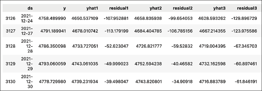
Figure 15.25: Preview of the DataFrame containing 10-step-ahead forecasts

This time, the DataFrame will contain 10 predictions for each row: yhat1, yhat2, …, yhat10. To learn how to interpret the table, we can look at the last row presented in Figure 15.25. The yhat2 value corresponds to the prediction for 2021-12-30, made 2 days prior to that date. So the number after yhat indicates the age of the prediction (in this case, expressed in days).

Alternatively, we can shift this around. By specifying raw=True while calling the predict method, we obtain predictions made on the row’s date, instead of a prediction for that date:

pred_df = model.predict(df, raw=True, decompose=False)
pred_df.tail()

Executing the snippet generated the following preview of the DataFrame:

Figure 15.26: Preview of the DataFrame containing the first 5 of the 10-step-ahead forecasts

We can easily track some forecasts in both tables to see how the tables’ structures differ.

When plotting a multi-step-ahead forecast, we will see multiple lines—each originating from a different date of the forecast:

pred_df = model.predict(df_test)
model.plot(pred_df)
ax = plt.gca()
ax.legend(loc='center left', bbox_to_anchor=(1, 0.5))
ax.set_title("10-day ahead multi-step forecast")

Executing the snippet generates the following plot:

Figure 15.27: 10-day-ahead multi-step forecast

The plot is quite hard to read due to the overlapping lines. We can highlight the forecast made for a certain step using the highlight_nth_step_ahead_of_each_forecast method. The following snippet illustrates how to do it:

model = model.highlight_nth_step_ahead_of_each_forecast(1)
model.plot(pred_df)
ax = plt.gca()
ax.set_title("Step 1 of the 10-day ahead multi-step forecast")

Executing the snippet generates the following plot:

Figure 15.28: Step 1 of the 10-day multi-step forecast

After analyzing Figure 15.28, we can conclude that the model is still struggling with the predictions and the forecasted values are very close to the last known values.

Other features

NeuralProphet also contains some other interesting features, including:

• Extensive cross-validation and benchmarking functionalities
• The components of the model such as holidays/events, seasonality, or future regressors do not need to be additive; they can also be multiplicative
• The default loss function is Huber loss, but we can change it to any of the other popular loss functions

See also

• Triebe, O., Laptev, N., & Rajagopal, R. 2019. Ar-net: A simple autoregressive neural network for time-series. arXiv preprint arXiv:1911.12436.
• Triebe, O., Hewamalage, H., Pilyugina, P., Laptev, N., Bergmeir, C., & Rajagopal, R. 2021. Neuralprophet: Explainable forecasting at scale. arXiv preprint arXiv:2111.15397.

Summary

In this chapter, we explored how we can use deep learning for both tabular and time series data. Instead of building the neural networks from scratch, we used modern Python libraries which handled most of the heavy lifting for us.

As we have already mentioned, deep learning is a rapidly developing field with new neural network architectures being published daily. Hence, it is difficult to scratch even just the tip of the iceberg in a single chapter. That is why we will now point you toward some of the popular and influential approaches/libraries that you might want to explore on your own.

Tabular data

Below we list some relevant papers and Python libraries that will definitely be good starting points for further exploration of the topic of using deep learning with tabular data.

Further reading:

• Huang, X., Khetan, A., Cvitkovic, M., & Karnin, Z. 2020. Tabtransformer: Tabular data modeling using contextual embeddings. arXiv preprint arXiv:2012.06678.
• Popov, S., Morozov, S., & Babenko, A. 2019. Neural oblivious decision ensembles for deep learning on tabular data. arXiv preprint arXiv:1909.06312.

Libraries:

• pytorch_tabular—this library offers a framework for using deep learning models for tabular data. It provides models such as TabNet, TabTransformer, FT Transformer, and a feed-forward network with category embedding.
• pytorch-widedeep—a library based on Google’s Wide and Deep algorithm. It not only allows us to use deep learning with tabular data but also facilitates the combination of text and images with corresponding tabular data.

Time series

In this chapter, we have covered two deep learning-based approaches to time series forecasting—DeepAR and NeuralProphet. We highly recommend also looking into the following resources on analyzing and forecasting time series.

Further reading:

• Chen, Y., Kang, Y., Chen, Y., & Wang, Z. (2020). “Probabilistic forecasting with temporal convolutional neural network”, Neurocomputing, 399: 491-501.
• Gallicchio, C., Micheli, A., & Pedrelli, L. 2018. “Design of deep echo state networks”, Neural Networks, 108: 33-47.
• Kazemi, S. M., Goel, R., Eghbali, S., Ramanan, J., Sahota, J., Thakur, S., ... & Brubaker, M. 2019. Time2vec: Learning a vector representation of time. arXiv preprint arXiv:1907.05321.
• Lea, C., Flynn, M. D., Vidal, R., Reiter, A., & Hager, G. D. 2017. Temporal convolutional networks for action segmentation and detection. In proceedings of the IEEE Conference on Computer Vision and Pattern Recognition, 156-165.
• Lim, B., Arık, S. Ö., Loeff, N., & Pfister, T. 2021. “Temporal fusion transformers for interpretable multi-horizon time series forecasting”, International Journal of Forecasting, 37(4): 1748-1764.
• Oreshkin, B. N., Carpov, D., Chapados, N., & Bengio, Y. 2019. N-BEATS: Neural basis expansion analysis for interpretable time series forecasting. arXiv preprint arXiv:1905.10437.

Libraries:

• tsai—this is a deep learning library built on top of PyTorch and fastai. It focuses on various time series-related tasks, including classification, regression, forecasting, and imputation. Aside from already traditional approaches such as LSTMs or GRUs, it implements a selection of state-of-the-art architectures such as ResNet, InceptionTime, TabTransformer, and Rocket.
• gluonts—a Python library for probabilistic time series modeling using deep learning. It contains models such as DeepAR, DeepVAR, N-BEATS, Temporal Fusion Transformer, WaveNet, and many more.
• darts—a versatile library for time series forecasting using a variety of methods, from statistical models such as ARIMA to deep neural networks. It contains implementations of models such as N-BEATS, Temporal Fusion Transformer, and temporal convolutional neural networks.

Other domains

In this chapter, we have focused on showing the applications of deep learning in tabular data and time series forecasting. However, there are many more use cases and recent developments. For example, FinBERT is a pre-trained NLP model used to analyze the sentiment of financial texts, such as earnings call transcripts.

On the other hand, we can use the recent developments in generative adversarial networks to generate synthetic data for our models. Below, we mention some interesting starting points for further exploration of the field of deep learning in a financial context.

Further reading:

• Araci, D. 2019. Finbert: Financial sentiment analysis with pre-trained language models. arXiv preprint arXiv:1908.10063.
• Cao, J., Chen, J., Hull, J., & Poulos, Z. 2021. “Deep hedging of derivatives using reinforcement learning”, The Journal of Financial Data Science, 3(1): 10-27.
• Xie, J., Girshick, R., & Farhadi, A. 2016, June. Unsupervised deep embedding for clustering analysis. In International conference on machine learning, 478-487. PMLR.
• Yoon, J., Jarrett, D., & Van der Schaar, M. 2019. Time-series generative adversarial networks. Advances in neural information processing systems, 32.

Libraries:

• tensortrade—offers a reinforcement learning framework for training, evaluating, and deploying trading agents.
• FinRL—an ecosystem consisting of various applications of reinforcement learning in the financial context. It covers state-of-the-art algorithms, financial applications such as crypto trading or high-frequency trading, and more.
• ydata-synthetic—a library useful for generating synthetic tabular and time series data with the use of state-of-the-art generative models, for example, TimeGAN.
• sdv—the name stands for Synthetic Data Vault and it is, as the name suggests, another library useful for generating synthetic data. It covers tabular, relational, and time series data.
• transformers—this is a Python library that allows us to access a range of pre-trained transformer models (for example, FinBERT). The company behind the library is called Hugging Face, and it offers a platform that enables its users to build, train, and deploy ML/DL models.
• autogluon—this library offers AutoML for tabular data, as well as text and images. It contains various state-of-the-art ML and DL models.

Join us on Discord!

To join the Discord community for this book – where you can share feedback, ask questions to the author, and learn about new releases – follow the QR code below:

https://packt.link/ips2H