4

Exploring Financial Time Series Data

In the previous chapters, we learned how to preprocess and visually explore financial time series data. This time, we will use algorithms and/or statistical tests to automatically identify potential issues (like outliers) and analyze the data for the existence of trends or other patterns (for example, mean-reversion).

We will also dive deeper into the stylized facts of asset returns. Together with outlier detection, those recipes are particularly important when working with financial data. When we want to build models/strategies based on asset prices, we have to make sure that they can accurately capture the dynamics of the returns.

Having said that, most of the techniques described in this chapter are not restricted only to financial time series and can be effectively used in other domains as well.

In this chapter, we will cover the following recipes:

• Outlier detection using rolling statistics
• Outlier detection with the Hampel filter
• Detecting changepoints in time series
• Detecting trends in time series
• Detecting patterns in a time series using the Hurst exponent
• Investigating stylized facts of asset returns

Outlier detection using rolling statistics

While working with any kind of data, we often encounter observations that are significantly different from the majority, that is, outliers. In the financial domain, they can be the result of a wrong price, something major happening in the financial markets, or an error in the data processing pipeline. Many machine learning algorithms and statistical approaches can be heavily influenced by outliers, leading to incorrect/biased results. That is why we should identify and handle the outliers before creating any models.

In this recipe, we cover a relatively simple, filter-like approach to detect outliers based on the rolling average and standard deviation. We will use Tesla’s stock prices from the years 2019 to 2020.

How to do it…

Execute the following steps to detect outliers using the rolling statistics and mark them on the plot:

1. Import the libraries:

   import pandas as pd
   import yfinance as yf
   
2. Download Tesla’s stock prices from 2019 to 2020 and calculate simple returns:

   df = yf.download("TSLA",
                    start="2019-01-01",
                    end="2020-12-31",
                    progress=False)
   df["rtn"] = df["Adj Close"].pct_change()
   df = df[["rtn"]].copy()
   
3. Calculate the 21-day rolling mean and standard deviation:

   df_rolling = df[["rtn"]].rolling(window=21) 
                           .agg(["mean", "std"])
   df_rolling.columns = df_rolling.columns.droplevel()
   
4. Join the rolling data back to the initial DataFrame:

   df = df.join(df_rolling)
   
5. Calculate the upper and lower thresholds:

   N_SIGMAS = 3
   df["upper"] = df["mean"] + N_SIGMAS * df["std"]
   df["lower"] = df["mean"] - N_SIGMAS * df["std"]
   
6. Identify the outliers using the previously calculated thresholds:

   df["outlier"] = (
       (df["rtn"] > df["upper"]) | (df["rtn"] < df["lower"])
   )
   
7. Plot the returns together with the thresholds and mark the outliers:

   fig, ax = plt.subplots()
   df[["rtn", "upper", "lower"]].plot(ax=ax)
   ax.scatter(df.loc[df["outlier"]].index,
              df.loc[df["outlier"], "rtn"],
              color="black", label="outlier")
   ax.set_title("Tesla's stock returns")
   ax.legend(loc="center left", bbox_to_anchor=(1, 0.5))
   plt.show()
   

   Running the snippet generates the following plot:

Figure 4.1: Outliers identified using the filtering algorithm

In the plot, we can observe outliers marked with a black dot, together with the thresholds used for determining them. One thing to notice is that when there are two large (in absolute terms) returns in the vicinity of one another, the algorithm identifies the first one as an outlier and the second one as a regular observation. This might be due to the fact that the first outlier enters the rolling window and affects the moving average/standard deviation. We can observe a situation like that in the first quarter of 2020.

How it works…

After importing the libraries, we downloaded Tesla’s stock prices, calculated the returns, and only kept a single column — the one with the returns — for further analysis.

To identify the outliers, we started by calculating the moving statistics using a 21-day rolling window. We used 21 as this is the average number of trading days in a month, and in this example, we work with daily data. However, we can choose different values, and then the moving average will react more quickly/slowly to changes. We can also use the (exponentially) weighted moving average if we find it more meaningful for our particular case. To implement the moving metrics, we used the combination of the rolling and agg methods of a pandas DataFrame. After calculating the statistics, we dropped one level of the MultiIndex to simplify the analysis.

In Step 4, we joined the rolling statistics back to the original DataFrame. Then, we created additional columns containing the upper and lower decision thresholds. We decided to use 3 standard deviations above/below the rolling average as the boundaries. Any observation lying beyond them was considered an outlier. We should keep in mind that the logic of the filtering algorithm is based on the assumption of the stock returns being normally distributed. Later in the chapter, we will see that this assumption does not hold empirically. We coded that condition as a separate column in Step 6.

In the last step, we visualized the returns series, along with the upper/lower decision thresholds, and marked the outliers with a black dot. To make the plot more readable, we moved the legend outside of the plotting area.

In real-life cases, we should not only identify the outliers but also treat them, for example, by capping them at the maximum/minimum acceptable value, replacing them with interpolated values, or by following any of the other possible approaches.

There’s more…

Defining functions

In this recipe, we demonstrated how to carry out all the steps required for identifying the outliers as separate operations on the DataFrame. However, we can quickly encapsulate all of the steps into a single function and make it generic to handle more use cases. You can find an example of how to do so below:

def identify_outliers(df, column, window_size, n_sigmas):
    """Function for identifying outliers using rolling statistics"""
    
    df = df[[column]].copy()
    df_rolling = df.rolling(window=window_size) 
                   .agg(["mean", "std"])
    df_rolling.columns = df_rolling.columns.droplevel()
    df = df.join(df_rolling)
    df["upper"] = df["mean"] + n_sigmas * df["std"]
    df["lower"] = df["mean"] - n_sigmas * df["std"]
    
    return ((df[column] > df["upper"]) | (df[column] < df["lower"]))

The function returns a pd.Series containing Boolean flags indicating whether a given observation is an outlier or not. An additional benefit of using a function is that we can easily experiment with using different parameters (such as window sizes and the numbers of standard deviations used for creating the thresholds).

Winsorization

Another popular approach for treating outliers is winsorization. It is based on replacing outliers in data to limit their effect on any potential calculations. It’s easier to understand winsorization using an example. A 90% winsorization results in replacing the top 5% of values with the 95th percentile. Similarly, the bottom 5% is replaced using the value of the 5th percentile. We can find the corresponding winsorize function in the scipy library.

Outlier detection with the Hampel filter

We will cover one more algorithm used for outlier detection in time series—the Hampel filter. Its goal is to identify and potentially replace outliers in a given series. It uses a centered sliding window of size 2x (given x observations before/after) to go over the entire series.

For each of the sliding windows, the algorithm calculates the median and the median absolute deviation (a form of a standard deviation).

Similar to the previously covered algorithm, we treat an observation as an outlier if it differs from the window’s median by more than a determined number of standard deviations. We can then replace such an observation with the window’s median.

We can experiment with the different settings of the algorithm’s hyperparameters. For example, a higher standard deviation threshold makes the filter more forgiving, while a lower one results in more data points being classified as outliers.

In this recipe, we will use the Hampel filter to see if any observations in a time series of Tesla’s prices from 2019 to 2020 can be considered outliers.

How to do it…

Execute the following steps to identify outliers using the Hampel filter:

1. Import the libraries:

   import yfinance as yf
   from sktime.transformations.series.outlier_detection import HampelFilter
   
2. Download Tesla’s stock prices from the years 2019 to 2020 and calculate simple returns:

   df = yf.download("TSLA",
                    start="2019-01-01",
                    end="2020-12-31",
                    progress=False)
   df["rtn"] = df["Adj Close"].pct_change()
   
3. Instantiate the HampelFilter class and use it for detecting the outliers:

   hampel_detector = HampelFilter(window_length=10, 
                                  return_bool=True)
   df["outlier"] = hampel_detector.fit_transform(df["Adj Close"])
   
4. Plot Tesla’s stock price and mark the outliers:

   fig, ax = plt.subplots()
   df[["Adj Close"]].plot(ax=ax)
   ax.scatter(df.loc[df["outlier"]].index,
              df.loc[df["outlier"], "Adj Close"],
              color="black", label="outlier")
   ax.set_title("Tesla's stock price")
   ax.legend(loc="center left", bbox_to_anchor=(1, 0.5))
   plt.show()
   

   Running the code generates the following plot:

Figure 4.2: Tesla’s stock prices and the outliers identified using the Hampel filter

Using the Hampel filter, we identified seven outliers. At first glance, it might be interesting and maybe even a bit counterintuitive that the biggest spike and drop around September 2020 were not detected, but some smaller jumps later on were. We have to remember that this filter uses a centered window, so while looking into the observation at the peak of the spike, the algorithm also looks at the previous and next five observations, which include high values as well.

How it works…

The first two steps are quite standard—we imported the libraries, downloaded the stock prices, and calculated simple returns.

In Step 3, we instantiated the object of the HampelFilter class. We used the filter’s implementation from the sktime library, which we will also explore further in Chapter 7, Machine Learning-Based Approaches to Time Series Forecasting. We specified that we want to use a window of length 10 (5 observations before and 5 after) and for the filter to return a Boolean flag whether the observation is an outlier or not. The default setting of return_bool will return a new series in which the outliers will be replaced with NaNs. That is because the authors of sktime suggest using the filter for identifying and removing the outliers, and then using a companion Imputer class for filling in the missing values.

sktime uses methods similar to those available in scikit-learn, so we first need to fit the transformer object to the data and then transform it to obtain the flag indicating whether the observation is an outlier. Here, we completed two steps at once by using the fit_transform method applied to the adjusted close price.

In the last step, we plotted the stock price as a line plot and marked the outliers as black dots.

There’s more…

For comparison’s sake, we can also apply the very same filter to the returns calculated using the adjusted close prices. This way, we can see if the algorithm will identify different observations as outliers:

1. Identify the outliers among the stock returns:

   df["outlier_rtn"] = hampel_detector.fit_transform(df["rtn"])
   

   Because we have already instantiated the HampelFilter, we do not need to do it again. We can just fit it to the new data (returns) and transform it to get the Boolean flag.

2. Plot Tesla’s daily returns and mark the outliers:

   fig, ax = plt.subplots()
   df[["rtn"]].plot(ax=ax)
   ax.scatter(df.loc[df["outlier_rtn"]].index,
              df.loc[df["outlier_rtn"], "rtn"],
              color="black", label="outlier")
   ax.set_title("Tesla's stock returns")
   ax.legend(loc="center left", bbox_to_anchor=(1, 0.5))
   plt.show()
   

   Running the code generates the following plot:

   

   Figure 4.3: Tesla’s stock returns and the outliers identified using the Hampel filter

   We can immediately see that the algorithm detected more outliers when using the returns instead of the prices.

3. Investigate the overlap in outliers identified for the prices and returns:

   df.query("outlier == True and outlier_rtn == True")
   

Figure 4.4: The date that was identified as an outlier using both prices and returns

There is only a single date that was identified as an outlier based on both prices and returns.

See also

Anomaly/outlier detection is an entire field in data science, and there are numerous approaches to identifying suspicious observations. We have covered two algorithms that are especially suitable for time series problems. However, there are many possible approaches to anomaly detection in general. We will cover outlier detection methods used for data other than time series in Chapter 13, Applied Machine Learning: Identifying Credit Default. Some of them can also be used for time series.

Here are a few interesting anomaly/outlier detection libraries:

• https://github.com/datamllab/tods
• https://github.com/zillow/luminaire/
• https://github.com/signals-dev/Orion
• https://pycaret.org/anomaly-detection/
• https://github.com/linkedin/luminol—a library created by LinkedIn; unfortunately, it is not actively maintained anymore
• https://github.com/twitter/AnomalyDetection—this R package (created by Twitter) is quite famous and was ported to Python by some individual contributors

A few more references:

• Hampel F. R. 1974. “The influence curve and its role in robust estimation.” Journal of the American Statistical Association, 69: 382-393—a paper introducing the Hampel filter
• https://www.sktime.org/en/latest/index.html—documentation of sktime

Detecting changepoints in time series

A changepoint can be defined as a point in time when the probability distribution of a process or time series changes, for example, when there is a change to the mean in the series.

In this recipe, we will use the CUSUM (cumulative sum) method to detect shifts of the means in a time series. The implementation used in the recipe has two steps:

1. Finding the changepoint—an iterative process is started by first initializing a changepoint in the middle of the given time series. Then, the CUSUM approach is carried out based on the selected point. The following changepoint is located where the previous CUSUM time series is either maximized or minimized (depending on the direction of the changepoint we want to locate). We continue this process until a stable changepoint is located or we exceed the maximum number of iterations.
2. Testing its statistical significance—a log-likelihood ratio test is used to test if the mean of the given time series changes at the identified changepoint. The null hypothesis states that there is no change in the mean of the series.

Some further remarks about the implementation of the algorithm:

• The algorithm can be used to detect both upward and downward shifts.
• The algorithm can find at most one upward and one downward changepoint.
• By default, the changepoints are only reported if the null hypothesis is rejected.
• Under the hood, the Gaussian distribution is used to calculate the CUSUM time series value and perform the hypothesis test.

In this recipe, we will apply the CUSUM algorithm to identify changepoints in Apple’s stock prices from 2020.

How to do it…

Execute the following steps to detect changepoints in Apple’s stock price:

1. Import the libraries:

   import yfinance as yf
   from kats.detectors.cusum_detection import CUSUMDetector
   from kats.consts import TimeSeriesData
   
2. Download Apple’s stock price from 2020:

   df = yf.download("AAPL",
                    start="2020-01-01",
                    end="2020-12-31",
                    progress=False)
   
3. Keep only the adjusted close price, reset the index, and rename the columns:

   df = df[["Adj Close"]].reset_index(drop=False)
   df.columns = ["time", "price"]
   
4. Convert the DataFrame into a TimeSeriesData object:

   tsd = TimeSeriesData(df)
   
5. Instantiate and run the changepoint detector:

   cusum_detector = CUSUMDetector(tsd)
   change_points = cusum_detector.detector(
       change_directions=["increase"]
   )
   cusum_detector.plot(change_points)
   

   Running the code generates the following plot:

   

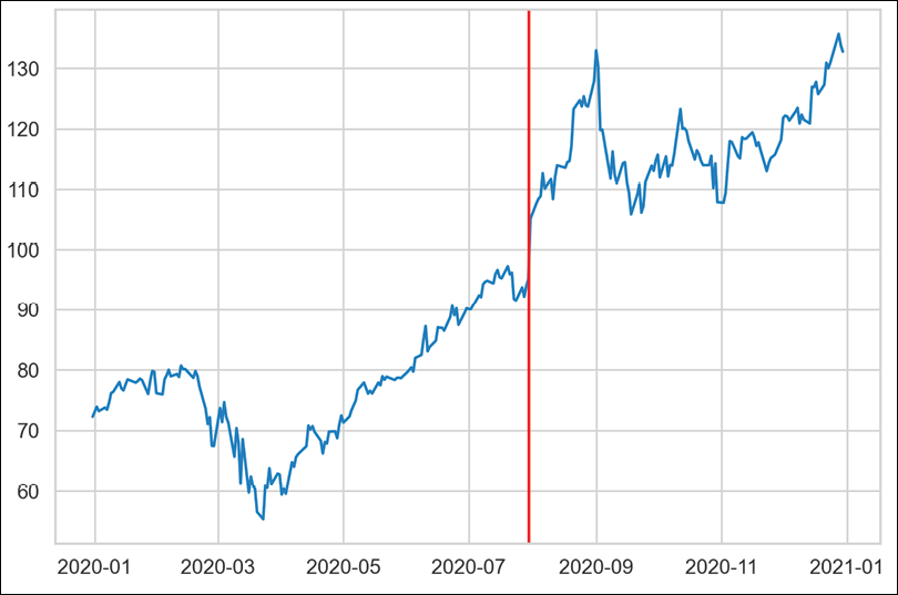
   Figure 4.5: The changepoint detected by the CUSUM algorithm

   We see that the algorithm picked the biggest jump as the changepoint.

6. Investigate the detected changepoint in more detail:

   point, meta = change_points[0]
   point
   

   What returns the following information about the detected changepoint:

   TimeSeriesChangePoint(start_time: 2020-07-30 00:00:00, end_time: 2020-07-30 00:00:00, confidence: 1.0)
   

The identified changepoint is on the 30th of July and indeed the stock price jumped from $95.4 on that day to $105.4 on the next day, mostly due to a strong quarterly earnings report.

How it works…

In the first step, we imported the libraries. For detecting the changepoints, we used the kats library from Facebook. Then, we fetched Apple’s stock prices from 2020. For this analysis, we used the adjusted close prices.

To work with kats, we need to have our data in a particular format. That is why in Step 3, we only kept the adjusted close prices, reset the index without dropping it (as we need that column), and renamed the columns. One thing to remember is that the column containing the dates/datetimes must be called time. In Step 4, we converted the DataFrame into a TimeSeriesData object, which is a representation used by kats.

In Step 5, we instantiated the CUSUMDetector using the previously created data. We did not change any default settings. Then, we identified the changepoints using the detector method. For this analysis, we were only interested in increases, so we specified the change_directions argument. Lastly, we plotted the detected changepoint using the plot method of the cusum_detector object. One thing to note here is that we had to provide the identified changepoints as input for the method.

In the very last step, we looked further into the detected changepoints. The returned object is a list containing two elements: the TimeSeriesChangePoint object containing information, such as the date of the identified changepoint and the algorithm’s confidence, and a metadata object. By using the latter’s __dict__ method, we can access more information about the point: the direction, the mean before/after the changepoint, the p-value of the likelihood ratio test, and more.

There’s more…

The library offers quite a few more interesting functionalities regarding changepoint detection. We will only cover two of them, and I highly encourage you to explore them further on your own.

Restricting the detection window

The first one is to restrict the window in which we want to look for the changepoint. We can do so using the interest_window argument of the detector method. Below, we only looked for a changepoint between the 200th and 250th observations (reminder: this is a trading year and not a full calendar year, so there are only around 252 observations).

Narrow down the window in which we want to search for the changepoint:

change_points = cusum_detector.detector(change_directions=["increase"],
                                        interest_window=[200, 250])
cusum_detector.plot(change_points)

We can see the modified results in the following plot:

Figure 4.6: Changepoint identified between the 200^th and 250^th observations in the series

Aside from the identified changepoint, we can also see the window we have selected.

Using different changepoint detection algorithms

The kats library also contains other interesting algorithms for changepoint detection. One of them is RobustStatDetector. Without going into too much detail about the algorithm itself, it smoothens the data using moving averages before identifying the points of interest. Another interesting feature of the algorithm is that it can detect multiple changepoints in a single run.

Use another algorithm to detect changepoints (RobustStatDetector):

from kats.detectors.robust_stat_detection import RobustStatDetector
robust_detector = RobustStatDetector(tsd)
change_points = robust_detector.detector()
robust_detector.plot(change_points)

Running the snippet generates the following plot:

Figure 4.7: Identifying changepoints using the RobustStatDetector

This time, the algorithm picked up two additional changepoints compared to the previous attempt.

See also

• https://github.com/facebookresearch/Kats—the GitHub repository of Facebook’s Kats
• Page, E. S. 1954. “Continuous inspection schemes.” Biometrika 41(1): 100–115
• Adams, R. P., & MacKay, D. J. (2007). Bayesian online changepoint detection. arXiv preprint arXiv:0710.3742

Detecting trends in time series

In the previous recipe, we covered changepoint detection. Another class of algorithms can be used for trend detection, that is, identifying significant and prolonged changes in time series.

The kats library offers a trend detection algorithm based on the non-parametric Mann-Kendall (MK) test. The algorithm iteratively conducts the MK test on windows of a specified size and returns the starting points of each window for which this test turned out to be statistically significant.

To detect whether there is a significant trend in the window, the test inspects the monotonicity of the increases/decreases in the time series rather than the magnitude of the change in values. The MK test uses a test statistic called Kendall’s Tau, and it ranges from -1 to 1. We can interpret the values as follows:

• -1 indicates a perfectly monotonic decline
• 1 indicates a perfectly monotonic increase
• 0 indicates that there is no directional trend in the series

By default, the algorithm will only return periods in which the results were statistically significant.

You might be wondering why use an algorithm for detecting trends when it is easy to see them on the plot? That is very true; however, we should remember that the goal of using those algorithms is to look at more than a single series and time period at a time. We want to be able to detect trends at scale, for example, finding upward trends within hundreds of time series.

In this recipe, we will use the trend detection algorithm to investigate whether there were periods with significant increasing trends in NVIDIA’s stock prices from 2020.

How to do it…

Execute the following steps to detect increasing trends in NVIDIA’s stock prices from 2020:

1. Import the libraries:

   import yfinance as yf
   from kats.consts import TimeSeriesData
   from kats.detectors.trend_mk import MKDetector
   
2. Download NVIDIA’s stock prices from 2020:

   df = yf.download("NVDA",
                    start="2020-01-01",
                    end="2020-12-31",
                    progress=False)
   
3. Keep only the adjusted close price, reset the index, and rename the columns:

   df = df[["Adj Close"]].reset_index(drop=False)
   df.columns = ["time", "price"]
   
4. Convert the DataFrame into a TimeSeriesData object:

   tsd = TimeSeriesData(df)
   
5. Instantiate and run the trend detector:

   trend_detector = MKDetector(tsd, threshold=0.9)
   time_points = trend_detector.detector(
       direction="up", 
       window_size=30
   )
   
6. Plot the detected time points:

   trend_detector.plot(time_points)
   

   Running the line results in the following plot:

Figure 4.8: The identified starting points of upward trends

In Figure 4.8, we can see a lot of periods with some gaps in between. What is important to know is that the red vertical bars are not the detected windows, but rather a lot of detected trend starting points right next to each other. Running the selected configuration of the algorithm on our data resulted in identifying 95 periods of an increasing trend, which clearly have a lot of overlap.

How it works…

The first four steps are very similar to the previous recipe, with the only difference being that this time we downloaded NVIDIA’s stock price from 2020. Please refer to the previous recipe for more information about preparing the data for working with the kats library.

In Step 5, we instantiated the trend detector (MKDetector class) while providing the data and changing the threshold of the Tau coefficient to 0.9. This way, we obtain only the periods with higher trend intensity. Then, we used the detector method to find the time points. We were interested in increasing trends (direction="up") over a window of 30 days.

In Step 6, we plotted the results. We can also inspect in detail each of the 95 detected points. The returned time_points object is a list of tuples, in which each tuple contains the TimeSeriesChangePoint object (with the beginning date of the detected trend period) and the point’s metadata. In our case, we looked for periods of an increasing trend over a window of 30 days. Naturally, there will be quite an overlap in the periods of an increasing trend, as we identified multiple points, with each being the beginning of the period. As we can see in the plot, a lot of those identified points are consecutive.

See also

• Mann, H. B. 1945. “Non-Parametric Tests against Trend.” Econometrica 13: 245-259.
• Kendall, M. G. 1948. Rank Correlation Methods. Griffin.

Detecting patterns in a time series using the Hurst exponent

In finance, a lot of trading strategies are based on one of the following:

• Momentum—the investors try to use the continuance of the existing market trend to determine their positions
• Mean-reversion – the investors assume that properties such as stock returns and volatility will revert to their long-term average over time (also known as an Ornstein-Uhlenbeck process)

While we can relatively easily classify a time series as one of the two by inspecting it visually, this solution definitely does not scale well. That is why we can use approaches such as the Hurst exponent to identify if a given time series (not necessarily a financial one) is trending, mean-reverting, or simply a random walk.

Hurst exponent (H) is a measure for the long-term memory of a time series, that is, it measures the amount by which that series deviates from a random walk. The values of the Hurst exponent range between 0 and 1, with the following interpretation:

• H < 0.5—a series is mean-reverting. The closer the value is to 0, the stronger the mean-reversion process is.
• H = 0.5—a series is a geometric random walk.
• H > 0.5—a series is trending. The closer the value is to 1, the stronger the trend.

There are a few ways of calculating the Hurst exponent. In this recipe, we will focus on the one based on estimating the rate of the diffusive behavior, which is based on the variance of log prices. For the practical example, we will use 20 years of daily S&P 500 prices.

How to do it…

Execute the following steps to investigate whether S&P 500 prices are trending, mean-reverting, or an example of a random walk:

1. Import the libraries:

   import yfinance as yf
   import numpy as np
   import pandas as pd
   
2. Download S&P 500’s historical prices from the years 2000 to 2019:

   df = yf.download("^GSPC",
                    start="2000-01-01",
                    end="2019-12-31",
                    progress=False)
   df["Adj Close"].plot(title="S&P 500 (years 2000-2019)")
   

   Running the code generates the following plot:

   

   Figure 4.9: The S&P 500 index in the years 2000 to 2019

   We plot the data to get some initial intuition of what to expect from the calculated Hurst exponent.

3. Define a function calculating the Hurst exponent:

   def get_hurst_exponent(ts, max_lag=20):
       """Returns the Hurst Exponent of the time series"""
       lags = range(2, max_lag)
       tau = [np.std(np.subtract(ts[lag:], ts[:-lag])) for lag in lags]
       hurst_exp = np.polyfit(np.log(lags), np.log(tau), 1)[0]
       return hurst_exp
   
4. Calculate the values of the Hurst exponent using different values for the max_lag parameter:

   for lag in [20, 100, 250, 500, 1000]:
       hurst_exp = get_hurst_exponent(df["Adj Close"].values, lag)
       print(f"Hurst exponent with {lag} lags: {hurst_exp:.4f}")
   

   This returns the following:

   Hurst exponent with 20 lags: 0.4478
   Hurst exponent with 100 lags: 0.4512
   Hurst exponent with 250 lags: 0.4917
   Hurst exponent with 500 lags: 0.5265
   Hurst exponent with 1000 lags: 0.5180
   

   The more lags we include, the closer we get to the verdict that the S&P 500 series is a random walk.

5. Narrow down the data to the years 2005 to 2007 and calculate the exponents one more time:

   shorter_series = df.loc["2005":"2007", "Adj Close"].values
   for lag in [20, 100, 250, 500]:
       hurst_exp = get_hurst_exponent(shorter_series, lag)
       print(f"Hurst exponent with {lag} lags: {hurst_exp:.4f}")
   

   This returns the following:

   Hurst exponent with 20 lags: 0.3989
   Hurst exponent with 100 lags: 0.3215
   Hurst exponent with 250 lags: 0.2507
   Hurst exponent with 500 lags: 0.1258
   

It seems that the series from the 2005 to 2007 period is mean-reverting. For reference, the discussed time series is illustrated as follows:

Figure 4.10: The S&P 500 index in the years 2005 to 2007

How it works…

After importing the required libraries, we downloaded 20 years’ worth of daily S&P prices from Yahoo Finance. From looking at the plot, it is hard to say whether the time series is purely trending, mean-reverting, or a random walk. There seems to be a clear rising trend, especially in the second half of the series.

In Step 3, we defined a function used for calculating the Hurst exponent. For this approach, we need to provide the maximum number of lags to be used for the calculations. This parameter greatly impacts the results, as we will see later on.

The calculations of the Hurst exponent can be summarized in two steps:

1. For each lag in the considered range, we calculate the standard deviation of the differenced series (we will cover differencing in more depth in Chapter 6, Time Series Analysis and Forecasting).
2. Calculate the slope of the log plot of lags versus the standard deviations to get the Hurst exponent.

In Step 4, we calculated and printed the Hurst exponent for a range of different values of the max_lag parameter. For lower values of the parameter, the series could be considered slightly mean-reverting. While increasing the value of the parameter, the interpretation changed more in favor of the series being a random walk.

In Step 5, we carried out a similar experiment, but this time on a restricted time series. We only looked at data from the years 2005 to 2007. We also had to remove the max_lag of 1,000, given there were not enough observations in the restricted time series. As we could see, the results have changed a bit more drastically than before, from 0.4 for max_lag of 20 to 0.13 for 500 lags.

While using the Hurst exponent for our analyses, we should keep in mind that the results can vary depending on:

• The method we use for calculating the Hurst exponent
• The value of the max_lag parameter
• The period we are looking at – local patterns can be very different from the global ones

There’s more…

As we mentioned in the introduction, there are multiple ways to calculate the Hurst exponent. Another quite popular approach is to use the rescaled range (R/S) analysis. A brief literature review suggests that using the R/S statistic leads to better results in comparison to other methods such as the analysis of autocorrelations, variance ratios, and more. A possible shortcoming of that method is that it is very sensitive to short-range dependencies.

For an implementation of the Hurst exponent based on the rescaled range analysis, you can check out the hurst library.

See also

• https://github.com/Mottl/hurst—the repository of the hurst library
• Hurst, H. E. 1951. “Long-Term Storage Capacity of Reservoirs.” ASCE Transactions 116(1): 770–808
• Kroha, P., & Skoula, M. 2018, March. Hurst Exponent and Trading Signals Derived from Market Time Series. In ICEIS (1): 371–378

Investigating stylized facts of asset returns

Stylized facts are statistical properties that are present in many empirical asset returns (across time and markets). It is important to be aware of them because when we are building models that are supposed to represent asset price dynamics, the models should be able to capture/replicate these properties.

In this recipe, we investigate the five stylized facts using an example of daily S&P 500 returns from the years 2000 to 2020.

Getting ready

As this is a longer recipe with further subsections, we import the required libraries and prepare the data in this section:

1. Import the required libraries:

   import pandas as pd
   import numpy as np
   import yfinance as yf
   import seaborn as sns
   import scipy.stats as scs
   import statsmodels.api as sm
   import statsmodels.tsa.api as smt
   
2. Download the S&P 500 data and calculate the returns:

   df = yf.download("^GSPC", 
                    start="2000-01-01", 
                    end="2020-12-31",
                    progress=False)
    
   df = df[["Adj Close"]].rename(
       columns={"Adj Close": "adj_close"}
   )
   df["log_rtn"] = np.log(df["adj_close"]/df["adj_close"].shift(1))
   df = df[["adj_close", "log_rtn"]].dropna()
   

How to do it…

In this section, we sequentially investigate the five stylized facts in the S&P 500 returns series:

Fact 1: Non-Gaussian distribution of returns

It was observed in the literature that (daily) asset returns exhibit the following:

• Negative skewness (third moment): Large negative returns occur more frequently than large positive ones
• Excess kurtosis (fourth moment): Large (and small) returns occur more often than expected under normality

Run the following steps to investigate the existence of the first fact by plotting the histogram of returns and a quantile-quantile (Q-Q) plot:

1. Calculate the Normal probability density function (PDF) using the mean and standard deviation of the observed returns:

   r_range = np.linspace(min(df["log_rtn"]), 
                         max(df["log_rtn"]), 
                         num=1000)
   mu = df["log_rtn"].mean()
   sigma = df["log_rtn"].std()
   norm_pdf = scs.norm.pdf(r_range, loc=mu, scale=sigma)   
   
2. Plot the histogram and the Q-Q plot:

   fig, ax = plt.subplots(1, 2, figsize=(16, 8))
    
   # histogram
   sns.distplot(df.log_rtn, kde=False, 
                norm_hist=True, ax=ax[0])                                    
   ax[0].set_title("Distribution of S&P 500 returns", 
                   fontsize=16)                                                    
   ax[0].plot(r_range, norm_pdf, "g", lw=2, 
              label=f"N({mu:.2f}, {sigma**2:.4f})")
   ax[0].legend(loc="upper left")
    
   # Q-Q plot
   qq = sm.qqplot(df.log_rtn.values, line="s", ax=ax[1])
   ax[1].set_title("Q-Q plot", fontsize=16)
   plt.show()
   

   Executing the code results in the following plot:

Figure 4.11: The distribution of S&P 500 returns visualized using a histogram and a Q-Q plot

We can use the histogram (showing the shape of the distribution) and the Q-Q plot to assess the normality of the log returns. Additionally, we can print the summary statistics (please refer to the GitHub repository for the code):

---------- Descriptive Statistics ----------
Range of dates: 2000-01-03 – 2020-12-30
Number of observations: 5283
Mean: 0.0002
Median: 0.0006
Min: -0.1277
Max: 0.1096
Standard Deviation: 0.0126
Skewness: -0.3931
Kurtosis: 10.9531
Jarque-Bera statistic: 26489.07 with p-value: 0.00

By looking at the metrics such as the mean, standard deviation, skewness, and kurtosis, we can infer that they deviate from what we would expect under normality. The four moments of the Standard Normal distribution are 0, 1, 0, and 0 respectively. Additionally, the Jarque-Bera normality test gives us reason to reject the null hypothesis by stating that the distribution is normal at the 99% confidence level.

The fact that the returns do not follow the Normal distribution is crucial, given many statistical models and approaches assume that the random variable is normally distributed.

Fact 2: Volatility clustering

Volatility clustering is the pattern in which large changes in prices tend to be followed by large changes (periods of higher volatility), while small changes in price are followed by small changes (periods of lower volatility).

Run the following code to investigate the second fact by plotting the log returns series:

(
    df["log_rtn"]
    .plot(title="Daily S&P 500 returns", figsize=(10, 6))
)

Executing the code results in the following plot:

Figure 4.12: Examples of volatility clustering in the S&P 500 returns

We can observe clear clusters of volatility—periods of higher positive and negative returns. The fact that volatility is not constant and that there are some patterns in how it evolves is a very useful observation when we attempt to forecast volatility, for example, using GARCH models. For more information, please refer to Chapter 9, Modeling Volatility with GARCH Class Models.

Fact 3: Absence of autocorrelation in returns

Autocorrelation (also known as serial correlation) measures how similar a given time series is to the lagged version of itself over successive time intervals.

Below, we investigate the third fact by stating the absence of autocorrelation in returns:

1. Define the parameters for creating the autocorrelation plots:

   N_LAGS = 50
   SIGNIFICANCE_LEVEL = 0.05
   
2. Run the following code to create the autocorrelation function (ACF) plot of log returns:

   acf = smt.graphics.plot_acf(df["log_rtn"],
                               lags=N_LAGS,
                               alpha=SIGNIFICANCE_LEVEL)
   plt.show()
   

   Executing the snippet results in the following plot:

Figure 4.13: The plot of the autocorrelation function of the S&P 500 returns

Only a few values lie outside of the confidence interval (we do not look at lag 0) and can be considered statistically significant. We can assume that we have verified that there is no autocorrelation in the log-returns series.

Fact 4: Small and decreasing autocorrelation in squared/absolute returns

While we expect no autocorrelation in the return series, it was empirically proven that we can observe small and slowly decaying autocorrelation (also referred to as persistence) in simple nonlinear functions of the returns, such as absolute or squared returns. This observation is connected to the phenomenon we have already investigated, that is, volatility clustering.

The autocorrelation function of the squared returns is a common measure of volatility clustering. It is also referred to as the ARCH effect, as it is the key component of (G)ARCH models, which we cover in Chapter 9, Modeling Volatility with GARCH Class Models. However, we should keep in mind that this property is model-free and not exclusively connected to GARCH class models.

We can investigate the fourth fact by creating the ACF plots of squared and absolute returns:

fig, ax = plt.subplots(2, 1, figsize=(12, 10))
smt.graphics.plot_acf(df["log_rtn"]**2, lags=N_LAGS,
                      alpha=SIGNIFICANCE_LEVEL, ax=ax[0])
ax[0].set(title="Autocorrelation Plots",
          ylabel="Squared Returns")
smt.graphics.plot_acf(np.abs(df["log_rtn"]), lags=N_LAGS,
                      alpha=SIGNIFICANCE_LEVEL, ax=ax[1])
ax[1].set(ylabel="Absolute Returns",
          xlabel="Lag")
plt.show()

Executing the code results in the following plots:

Figure 4.14: The ACF plots of squared and absolute returns

We can observe the small and decreasing values of autocorrelation for the squared and absolute returns, which are in line with the fourth stylized fact.

Fact 5: Leverage effect

The leverage effect refers to the fact that most measures of an asset’s volatility are negatively correlated with its returns.

Execute the following steps to investigate the existence of the leverage effect in the S&P 500’s return series:

1. Calculate volatility measures as moving standard deviations:

   df["moving_std_252"] = df[["log_rtn"]].rolling(window=252).std()
   df["moving_std_21"] = df[["log_rtn"]].rolling(window=21).std()
   
2. Plot all the series:

   fig, ax = plt.subplots(3, 1, figsize=(18, 15),
                          sharex=True)
   df["adj_close"].plot(ax=ax[0])
   ax[0].set(title="S&P 500 time series",
             ylabel="Price ($)")
   df["log_rtn"].plot(ax=ax[1])
   ax[1].set(ylabel="Log returns")
   df["rolling_std_252"].plot(ax=ax[2], color="r",
                              label="Rolling Volatility 252d")
   df["rolling_std_21"].plot(ax=ax[2], color="g",
                              label="Rolling Volatility 21d")
   ax[2].set(ylabel="Moving Volatility",
             xlabel="Date")
   ax[2].legend()
   plt.show()
   

   We can now investigate the leverage effect by visually comparing the price series to the (rolling) volatility metric:

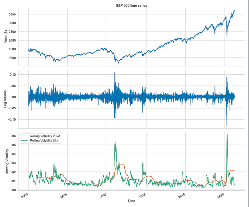
Figure 4.15: The rolling volatility metrics of the S&P 500 returns

In Figure 4.15, we can observe a pattern of increased volatility when the prices go down and decreased volatility when they are rising. This observation is in line with the fact’s definition.

How it works…

In this section, we describe the approaches we used to investigate the existence of the stylized facts in the S&P 500 log return series.

Fact 1: Non-Gaussian distribution of returns

We will break down investigating this fact into three parts.

Histogram of returns

The first step in investigating this fact was to plot a histogram by visualizing the distribution of returns. To do so, we used sns.distplot while setting kde=False (which does not use the Gaussian kernel density estimate) and norm_hist=True (this plot shows density instead of the count).

To see the difference between our histogram and Gaussian distribution, we superimposed a line representing the PDF of the Gaussian distribution with the mean and standard deviation coming from the considered return series.

First, we specified the range over which we calculated the PDF by using np.linspace (we set the number of points to 1,000; generally, the more points, the smoother the line) and then calculated the PDF using the scs.norm.pdf function. The default arguments correspond to the standard normal distribution, that is, with zero mean and unit variance. That is why we specified the loc and scale arguments as the sample mean and standard deviation, respectively.

To verify the existence of the previously mentioned patterns, we should look at the following:

• Negative skewness: The left tail of the distribution is longer, while the mass of the distribution is concentrated on the right-hand side of the distribution
• Excess kurtosis: Fat-tailed and peaked distribution

The second point is easier to observe on our plot, as there is a clear peak over the PDF, and we see more mass in the tails.

Q-Q plot

After inspecting the histogram, we looked at the Q-Q plot, on which we compared two distributions (theoretical and observed) by plotting their quantiles against each other. In our case, the theoretical distribution is Gaussian (normal), and the observed one comes from the S&P 500 returns.

To obtain the plot, we used the sm.qqplot function. If the empirical distribution is normal, then the vast majority of the points will lie on the red line. However, we see that this is not the case, as points on the left-hand side of the plot are more negative (that is, lower empirical quantiles are smaller) than expected in the case of the Gaussian distribution (indicated by the line). This means that the left tail of the returns distribution is heavier than that of the Gaussian distribution. Analogical conclusions can be drawn about the right tail, which is heavier than under normality.

Descriptive statistics

The last part involves looking at some statistics. We calculated them using the appropriate methods of pandas Series/DataFrames. We immediately saw that the returns exhibit negative skewness and excess kurtosis. We also ran the Jarque-Bera test (scs.jarque_bera) to verify that the returns do not follow a Gaussian distribution. With a p-value of zero, we rejected the null hypothesis that sample data has skewness and kurtosis matching those of a Gaussian distribution.

Fact 2: Volatility clustering

Another thing we should be aware of when investigating stylized facts is volatility clustering—periods of high returns alternating with periods of low returns, suggesting that volatility is not constant. To quickly investigate this fact, we plot the returns using the plot method of a pandas DataFrame.

Fact 3: Absence of autocorrelation in returns

To investigate whether there is significant autocorrelation in returns, we created the autocorrelation plot using plot_acf from the statsmodels library. We inspected 50 lags and used the default alpha=0.05, which means that we also plotted the 95% confidence interval. Values outside of this interval can be considered statistically significant.

Fact 4: Small and decreasing autocorrelation in squared/absolute returns

To verify this fact, we also used the plot_acf function from the statsmodels library. However, this time, we applied it to the squared and absolute returns.

Fact 5: Leverage effect

This fact states that most measures of asset volatility are negatively correlated with their returns. To investigate it, we used the moving standard deviation (calculated using the rolling method of a pandas DataFrame) as a measure of historical volatility. We used windows of 21 and 252 days, which correspond to one month and one year of trading data.

There’s more…

We present another method of investigating the leverage effect (fact 5). To do so, we use the VIX (CBOE Volatility Index), which is a popular metric of the stock market’s expectations regarding volatility. The measure is implied by option prices on the S&P 500 index. We take the following steps:

1. Download and preprocess the prices of the S&P 500 and VIX:

   df = yf.download(["^GSPC", "^VIX"],
                    start="2000-01-01",
                    end="2020-12-31",
                    progress=False)
   df = df[["Adj Close"]]
   df.columns = df.columns.droplevel(0)
   df = df.rename(columns={"^GSPC": "sp500", "^VIX": "vix"})
   
2. Calculate the log returns (we can just as well use simple returns):

   df["log_rtn"] = np.log(df["sp500"] / df["sp500"].shift(1))
   df["vol_rtn"] = np.log(df["vix"] / df["vix"].shift(1))
   df.dropna(how="any", axis=0, inplace=True)
   
3. Plot a scatterplot with the returns on the axes and fit a regression line to identify the trend:

   corr_coeff = df.log_rtn.corr(df.vol_rtn)
   ax = sns.regplot(x="log_rtn", y="vol_rtn", data=df,
                    line_kws={"color": "red"})
   ax.set(title=f"S&P 500 vs. VIX ($\rho$ = {corr_coeff:.2f})",
          ylabel="VIX log returns",
          xlabel="S&P 500 log returns")
   plt.show()
   

   We additionally calculated the correlation coefficient between the two series and included it in the title:

Figure 4.16: Investigating the relationship between the returns of S&P 500 and VIX

We can see that both the negative slope of the regression line and a strong negative correlation between the two series confirm the existence of the leverage effect in the return series.

See also

For more information, refer to the following:

• Cont, R. 2001. “Empirical properties of asset returns: stylized facts and statistical issues.” Quantitative Finance, 1(2): 223

Summary

In this chapter, we learned how to use a selection of algorithms and statistical tests to automatically identify potential patterns and issues (for example, outliers) in financial time series. With their help, we can scale up our analysis to an arbitrary number of assets instead of manually inspecting each and every time series.

We also explained the stylized facts of asset returns. These are crucial to understand, as many models or strategies assume a certain distribution of the variable of interest. Most frequently, a Gaussian distribution is assumed. And as we have seen, empirical asset returns are not normally distributed. That is why we have to take certain precautions to make our analyses valid while working with such time series.

In the next chapter, we will explore the vastly popular domain of technical analysis and see what insights we can gather from analyzing the patterns in asset prices.

Join us on Discord!

To join the Discord community for this book – where you can share feedback, ask questions to the author, and learn about new releases – follow the QR code below:

https://packt.link/ips2H