
Chapter 2. The R Environment
Now that R is downloaded and installed, it is time to get familiar with how to use R. The basic R interface on Windows is fairly Spartan as seen in Figure 2.1. The Mac interface (Figure 2.2) has some extra features and Linux has far fewer, being just a terminal.


Unlike other languages, R is very interactive. That is, results can be seen one command at a time. Languages such as C++ require that an entire section of code be written, compiled and run in order to see results. The state of objects and results can be seen at any point in R. This interactivity is one of the most amazing aspects of working with R.
There have been numerous Integrated Development Environments (IDEs) built for R. For the purposes of this book we will assume that RStudio is being used, which is discussed in Section 2.2.
2.1. Command Line Interface
The command line interface is what makes R so powerful, and also frustrating to learn. There have been attempts to build point-and-click interfaces for R, such as Rcmdr, but none have truly taken off. This is a testament to how typing in commands is much better than using a mouse. That might be hard to believe, especially for those coming from Excel, but over time it becomes easier and less error prone.
For instance, fitting a regression in Excel takes at least seven mouse clicks, often more: Data >> Data Analysis >> Regression >> OK >> Input Y Range >> Input X Range >> OK. Then it may need to be done all over again to make one little tweak or because there are new data. Even harder is walking a colleague through those steps via email. In contrast, the same command is just one line in R, which can easily be repeated and copied and pasted. This may be hard to believe initially, but after some time the command line makes life much easier.
To run a command in R, type it into the console next to the > symbol and press the Enter key. Entries can be as simple as the number 2 or complex functions, such as those seen in Chapter 8.
To repeat a line of code, simply press the Up Arrow key and hit Enter again. All previous commands are saved and can be accessed by repeatedly using the Up and Down Arrow keys to cycle through them.
Interrupting a command is done with Esc in Windows and Mac and Ctrl-C in Linux.
Often when working on a large analysis it is good to have a file of the code used. Until recently, the most common way to handle this was to use a text editor1 such as TextPad or UltraEdit to write code and then copy and paste it into the R console. While this worked, it was sloppy and led to a lot of switching between programs.
1. This means a programming text editor as opposed to a word processor such as Microsoft Word. A text editor preserves the structure of the text whereas word processors may add formatting that makes it unsuitable for insertion into the console.
2.2. RStudio
While there are a number of IDEs available, the best right now is RStudio, created by a team led by JJ Allaire whose previous products include ColdFusion and Windows Live Writer. It is available for Windows, Mac and Linux and looks identical in all of them. Even more impressive is the RStudio server, which runs an R instance on a Linux server and allows the user to run commands through the standard RStudio interface in a Web browser. It works with any version of R (greater than 2.11.1) including Revolution R from Revolution Analytics. RStudio has so many options that it can be a bit overwhelming. We will cover some of the most useful or frequently used features.
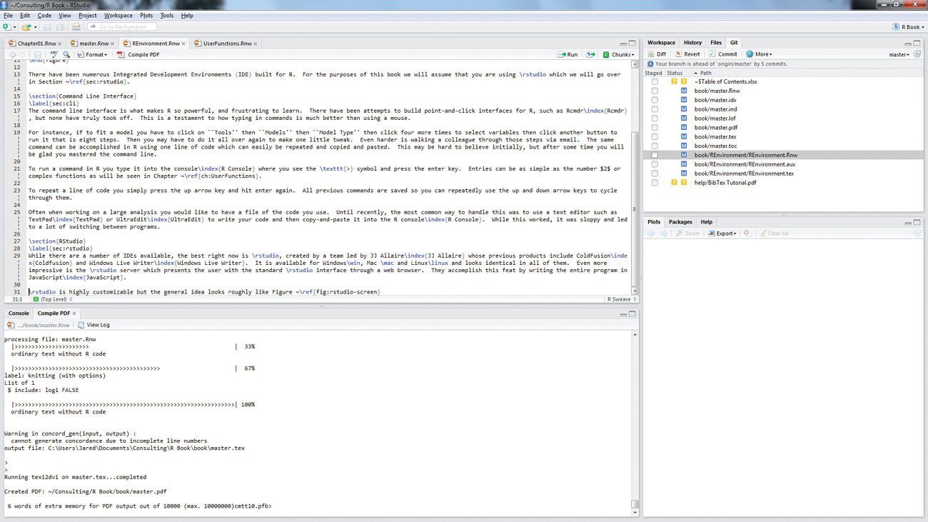
RStudio is highly customizable but the basic interface looks roughly like Figure 2.3. In this case the lower left pane is the R console, which can be used just like the standard R console. The upper left pane takes the place of a text editor but is far more powerful. The upper right pane holds information about the workspace, command history, files in the current folder and Git version control. The lower right pane displays plots, package information and help files.
There are a number of ways to send and execute commands from the editor to the console. To send one line place the cursor at the desired line and press Ctrl+Enter (Command+Enter on Mac). To insert a selection, simply highlight the selection and press Ctrl+Enter. To run an entire file of code, press Ctrl+Shift+S.
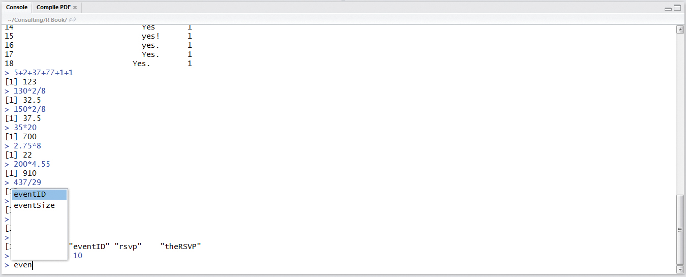
When typing code, such as an object name or function name, hitting Tab will autocomplete the code. If more than one object or function matches the letters typed so far, a dialog will pop up giving the matching options as shown in Figure 2.4.
Typing Ctrl+1 moves the cursor to the text editor area and Ctrl+2 moves it to the console. To move to the previous tab in the text editor, press Ctrl+Alt+Left in Windows, Ctrl+PageUp in Linux and Ctrl+Option+Left on Mac. To move to the next tab in the text editor, press Ctrl+Alt+Right in Windows, Ctrl+PageDown in Linux and Ctrl+Option+Right on Mac. For a complete list of shortcuts click Help >> Keyboard Shortcuts.
2.2.1. RStudio Projects
A primary feature of RStudio is projects. A project is a collection of files—and possibly data, results and graphs—that are all related to each other.2 Each package even has its own working directory. This is a great way to keep organized.
2. This is different from an R session, which is all the objects and work done in R and kept in memory for the current usage period, which usually resets upon restarting R.
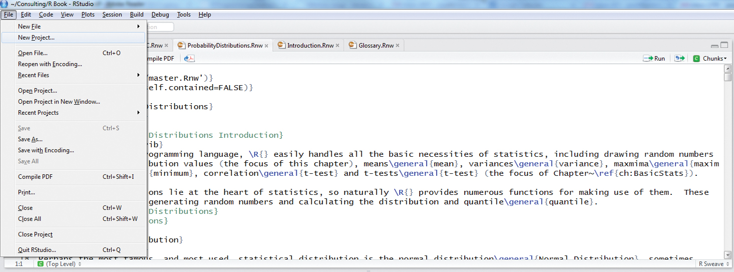
The simplest way to start a new project is to click File >> New Project as in Figure 2.5.
Three options are available, shown in Figure 2.6: starting a new project in a new directory, associating a project with an existing directory or checking out a project from a version control repository such as Git or SVN. In all three cases a .Rproj file is put into the resulting directory and keeps track of the project.

Figure 2.6 Three options are available to start a new project: a new directory, associating a project with an existing directory or checking out a project from a version control repository.
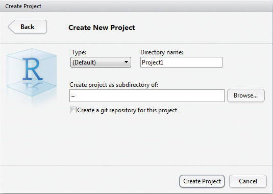
Choosing to create a new directory brings up a dialog, shown in Figure 2.7, that requests a project name and where to create a new directory.
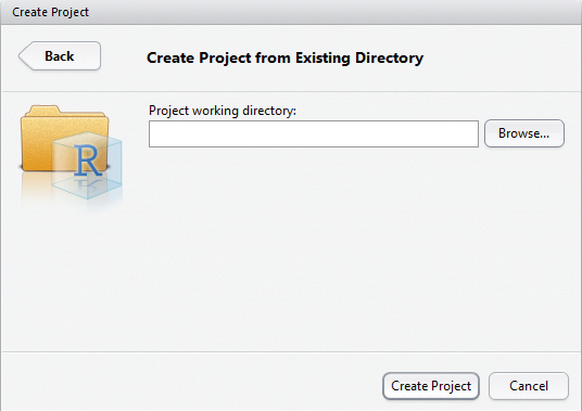
Choosing an existing directory asks for the name of the directory, seen in Figure 2.8.
Choosing to use version control (we prefer Git) firsts asks whether to use Git or SVN as in Figure 2.9.

Selecting Git asks for a repository URL, such as [email protected]:jaredlander/coefplot.git, which will then fill in the project directory name, as shown in Figure 2.10. As with creating a new directory, this will ask where to put this new directory.
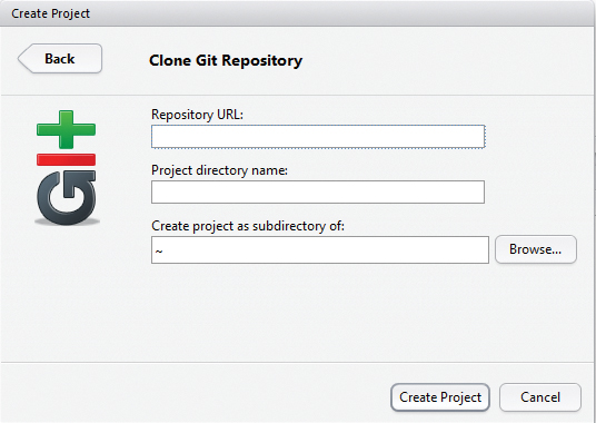
Figure 2.10 Enter the URL for a Git repository, as well as the folder where this should be cloned to.
2.2.2. RStudio Tools
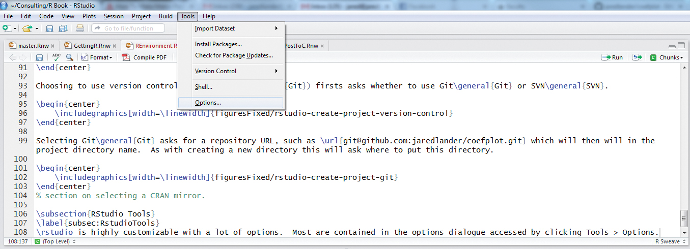
RStudio is highly customizable with a lot of options. Most are contained in the Options dialog accessed by clicking Tools >> Options, as seen in Figure 2.11.
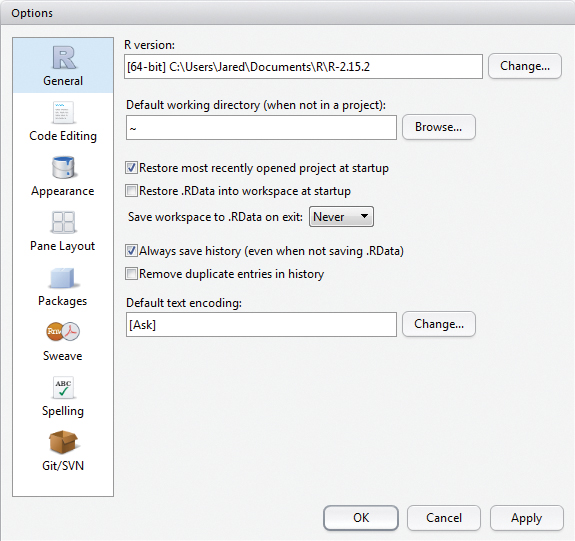
First are the General options, shown in Figure 2.12. There is a control for selecting which version of R to use. This is a powerful tool when a computer has a number of versions of R. However, RStudio must be restarted after changing the R version. In the future, RStudio is slated to offer the ability to set different versions of R for each project. It is also a good idea to not restore or save .RData files on startup and exiting.3
3. RData files are a convenient way of saving and sharing R objects and are discussed in Section 6.5.
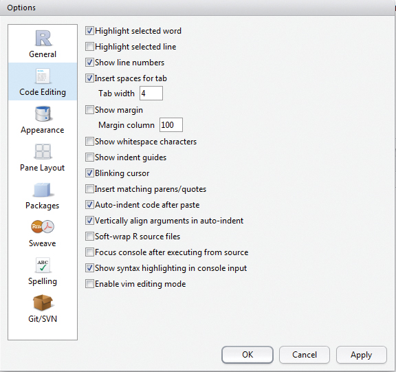
The Code Editing options, shown in Figure 2.13, control the way code is entered and displayed in the text editor. It is generally considered good practice to replace tabs with spaces, either two or four. Some hard-core programmers will appreciate vim mode. As of now there is no Emacs mode.
Appearance options, shown in Figure 2.14, change the way code looks, aesthetically. The font, size and color of the background and text can all be customized here.

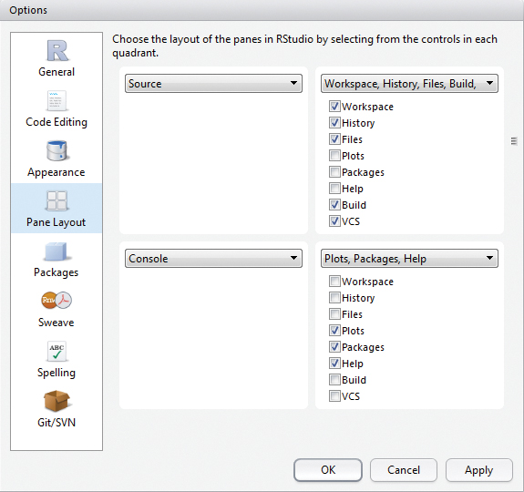
The Pane Layout options, shown in Figure 2.15, simply rearrange the panes that make up RStudio.
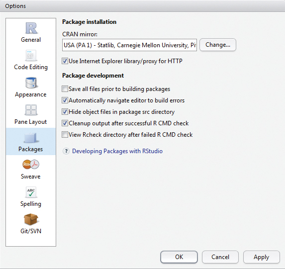
The Packages options, shown in Figure 2.16, set options regarding packages, although the most important is the CRAN mirror. While this is changeable from the console, this is the default setting. It is best to pick the mirror that is geographically the closest.
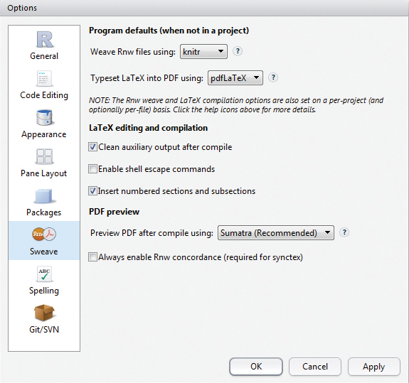
Sweave, Figure 2.17, may be a bit misnamed, as this is where to choose between using Sweave or knitr. Both are used for the generation of PDF documents with knitr also enabling the creation of HTML documents. knitr, detailed in Chapter 23, is by far the better option, although it must be installed first, which is explained in Section 3.1. This is also where the PDF viewer is selected.
RStudio contains a spelling checker for writing LATEX and Markdown documents (using knitr, preferably), which is controlled from the Spelling options, Figure 2.18. Not much needs to be set here.

Figure 2.18 These are the options for the spelling check dictionary, which allows language selection and the custom dictionaries.
The last option, Git/SVN, Figure 2.19, indicates where the executables for Git and SVN exist. This needs to be set only once but is necessary for version control.
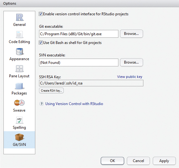
Figure 2.19 This is where to set the location of Git and SVN executables so they can be used by RStudio.
2.2.3. Git Integration
Using version control is a great idea for many reasons. First and foremost it provides snapshots of code at different points in time and can easily revert to those snapshots. Ancillary benefits include having a backup of the code and the ability to easily transfer the code between computers with little effort.
While SVN used to be the gold standard in version control it has since been superseded by Git, so that will be our focus. After associating a project with a Git repository4 RStudio has a pane for Git like the one shown in Figure 2.20.
4. A Git account should be set up with either GitHub (https://github.com/) or Bitbucket (https://bitbucket.org/) beforehand.

Figure 2.20 The Git pane shows the Git status of files under version control. A blue square with a white M indicates a file has been changed and needs to be committed. A yellow square with a white question mark indicates a new file that is not being tracked by Git.
The main functionality is committing changes, pushing them to the server and pulling changes made by other users. Clicking the Commit button brings up a dialog, Figure 2.21, which displays files that have been modified, or new files. Clicking on one of these files displays the changes; deletions are colored pink and additions are colored green. There is also a space to write a message describing the commit.
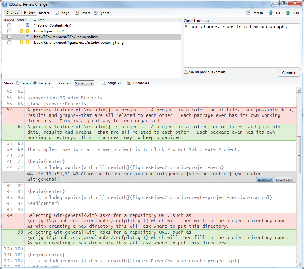
Figure 2.21 This displays files and the changes made to the files, with green being additions and pink being deletions. The upper right contains a space for writing commit messages.
Clicking Commit will stage the changes and clicking Push will send them to the server.
2.3. Revolution Analytics RPE
Revolution Analytics provides an IDE based on Visual Studio called the R Productivity Environment (RPE). The greatest benefit of the RPE is the visual debugger. If this feature is not needed,5 we recommend using Revolution with RStudio as the front-end, which can be set in the General options detailed in Section 2.2.2.
5. The latest version of RStudio now also offers a visual debugger.
2.4. Conclusion
R’s usability has greatly improved over the past few years, mainly thanks to Revolution Analytics’ RPE and RStudio. Using an IDE can greatly improve proficiency, and change working with R from merely tolerable to actually enjoyable.6 RStudio’s code completion, text editor, Git integration and projects are indispensable for a good programming work flow.
6. One of our students relayed that he preferred Matlab to R until he used RStudio.