15. Analysis of Covariance: Further Issues

The final chapter in this book builds on Chapter 14, “Analysis of Covariance: The Basics.” This chapter looks at some special considerations concerning the analysis of covariance, including a closer look at adjusting means using a covariate, multiple comparisons following a significant finding in ANCOVA, multiple covariates and factorial designs.

Adjusting Means with LINEST() and Effect Coding

There’s a special benefit to using LINEST() in conjunction with effect coding to run your ANCOVA. Doing so makes it much easier to obtain the adjusted means than using any traditional computation methods. Of course you want the adjusted means for their intrinsic interest—“What would my results have looked like if all the groups had begun with the same mean value on the covariate?” But you also want them because the F ratio from the ANCOVA might indicate one or more reliable differences among the adjusted group means. If so, you’ll want to carry out a multiple comparisons procedure to determine which adjusted means are reliably different. (See Chapter 10, “Testing Differences Between Means: The Analysis of Variance,” for a discussion of multiple comparisons following an ANOVA.)

Figure 15.1 shows the data and preliminary analysis for a study of auto tires. It is known that a tire’s age, even if it has just been sitting in a warehouse, contributes to its deterioration. One way to measure that deterioration is by checking for evidence of cracking on the tire’s exterior.

Figure 15.1. A visual scan of the data indicates that an ANCOVA would be a reasonable next step.

You decide to test whether the different types of stores that sell tires contribute to the deterioration of the tires, apart from that expected on the basis of the tires’ ages. You examine twelve different tires for the degree of deterioration as evidenced by the amount of surface cracking you can see. You examine four tires from each of three types of store: retailers that specialize in tires, auto dealers whose repair facilities sell tires, and repair garages. You come away with the findings shown in Figure 15.1.

By looking at the relationship between the mean degree of cracking and the mean tire age at each type of store, you can tell that as the age increases, so does the degree of cracking. You decide to test the mean differences in cracking among store types, using tire age as a covariate. The first step, as discussed in Chapter 14, is to check whether the regression coefficients between cracking and age are homogeneous in the three different groups. That test appears in Figure 15.2.

Figure 15.2. A data layout similar to this is needed for analysis by LINEST().

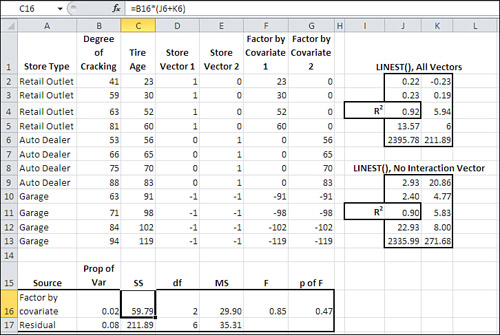
There are several aspects to note regarding the data in Figure 15.2.

The individual observations have been realigned in Figure 15.2 so that they occupy two columns, B and C: one for tire surface cracking and one for age. Figure 15.1 shows the data in two columns that span three different ranges, one range for each type of store (columns B, C, E, F, H, and I).

Four vectors have been added in Figure 15.2 from column D through column G. Columns D and E contain the familiar effect codes to indicate the type of store associated with each tire. The vectors in columns F and G are created by multiplying the covariate’s value by the value of each of the factor’s vectors. So, for example, cell F2 contains the product of cells C2 and D2, and cell G2 contains the product of cells C2 and E2.

The vectors in columns F and G represent the interaction between the factor, Store Type, and the covariate, Tire Age. Any variability in the outcome measure that the interaction vectors explain is due either to a real difference in the regression slopes between cracking and age in the different types of store, or to sampling error. The ANCOVA usually starts with a test of whether the regression lines differ at different levels of the factor.

To make that test, we use LINEST() twice. Each instance returns the amount of variability in the outcome measure, or R², that’s explained by the following:

• The full model (covariate, factor, and factor-covariate interaction)

• The restricted model (covariate and factor only)

The difference in the two measures of explained variance is attributable to the factor-covariate interaction. In Figure 15.2, the instance of LINEST() for the full model is in the range J2:K6. The cell with the R² is labeled accordingly, and shows that 0.92, or 92%, of the variance in the outcome measure is explained by all five predictor vectors.

By comparison, the instance of LINEST() in the range J9:K13 represents the restricted model and omits the interaction vectors in columns F and G from the analysis. The R² in cell J11 is 0.90, so the covariate and the factor vectors alone account for 90% of the variance in the outcome measure. Therefore, the interaction of the covariate with the factor accounts for a scant 2% of the variance in the outcome.

Despite the fact that so little variance is attributable to the interaction, it’s best to complete the analysis. That’s done in the range A16:G17 of Figure 15.2. There you can find a traditional ANOVA summary that tests the 2% of variance explained by the factor-covariate interaction against the residual variance. (You can get the residual proportion of variance by subtracting the R² in cell J4 from 1.0. Equivalently, you can get the residual sum of squares from cell K6.)

Notice from the p-value in cell G16 that this F ratio with 2 and 6 degrees of freedom can be expected by chance about half the time. Therefore, we retain the assumption that the regression slope of the outcome variable on the covariate is the same in each store type, in the population, and that any differences among the three regression coefficients is merely sampling error.

The next step is to perform the ANCOVA on the Tire Age covariate and the Store Type factor. Figure 15.3 shows that analysis.

Figure 15.3. The relationships between the covariate and the outcome, and between the factor and the outcome, are both reliable.

Two instances of LINEST() are needed in Figure 15.3 to test the relationship between the covariate and the outcome measure, and between the factor plus the covariate, and the outcome measure.

The range H2:I6 shows the first two columns of a LINEST() analysis of the regression of the outcome measure on the covariate and on the two factor vectors. Cell H4 shows that 0.90 of the variance in the outcome variable is explained by the covariate and the factor. (This analysis is of course identical to the one shown in J9:K13 of Figure 15.2.)

The second instance of LINEST() in Figure 15.3, in H9:I13, shows the regression of the outcome variable on the covariate only. The covariate explains 0.60 of the variability in the outcome measure, as shown in cell H11. Note that this figure, 0.60 or 60%, is repeated in cell B16 as part of the full ANCOVA analysis.

The difference between the R² for the covariate and the factor, and the R² for the covariate alone, is 0.29, or 29% of the variance in the outcome measure. This difference is attributable to the factor, Store Type.

The sums of squares in the range C16:C18 contribute little to the analysis—including them works out to little more than multiplying and dividing by the same constant when the F ratio is computed. But it’s traditional to include them.

The degrees of freedom are counted as discussed several times in Chapter 14. The covariate accounts for 1 df and the factor accounts for as many df as there are levels, minus 1. (It is not accidental that the number of vectors for each source of variation is equal to the number of df for that source.) The residual degrees of freedom is the total number of observations, less the number of covariates and factor vectors, less 1. Here, that’s 12 − 3 − 1, or 8.

As usual, dividing the sum of squares by the degrees of freedom results in the mean squares. The ratio of the mean square for the covariate to the mean square residual gives the F ratio for the covariate; the F ratio for the factor is, similarly, the result of dividing the mean square for the factor by the mean square for the residual.

(You could dispense with the sums of squares, divide the proportion of variance explained by the associated df, and form the same F ratios using the results of those divisions. This method is discussed in Testing for a Common Regression Line, in Chapter 14.)

An F ratio for the Store factor of 11.2 (see cell F17 in Figure 15.3) with 2 and 8 df occurs by chance, due to sampling error, 1% of the time (cell G17). Therefore, there is a reliable difference somewhere in the adjusted means. With only two means, it would be obvious where to look for a significant difference. With three or more means, it’s more complicated. For example, one mean might be significantly different from the other two, which are not significantly different. Or all three means might differ significantly. With four or more groups, the possibilities become more complex yet, and include questions such as whether the average of two group means is significantly different from the average of two other group means. These kinds of considerations, and their solutions, are discussed in Chapter 10, in the section titled “Multiple Comparison Procedures.”

But what you’re interested in, following an ANCOVA that returns a significantly large F ratio for a factor, is comparing the adjusted means. Because multiple comparisons involve the use of residual (also known as within-cell) variance, some modification is needed to account for the variation associated with the covariate.

In Chapter 14, one way to obtain adjusted group means in Excel was discussed. That was done in order to provide conceptual background for the procedure. But there is an easier way, provided you’re using LINEST() and effect coding to represent group membership (as this book has done for the preceding three chapters). We’ll cover that method next.

Effect Coding and Adjusted Group Means

Figure 15.4 shows again how to arrive at adjusted group means using traditional methods following a significant F ratio in an ANCOVA.

Figure 15.4. These figures represent the recommended calculations to adjust group means using the covariate in a traditional ANCOVA.

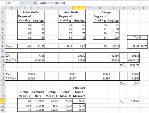
A lot of work must be done if you’re using traditional approaches to running an analysis of covariance. In Figure 15.4, the following tasks are illustrated:

• The unadjusted group means for the outcome measure (tire cracking) and the covariate (tire age), along with the grand mean for both variables, are calculated and shown in row 8.

• For each group, the sum of the squares of the covariate is found (row 10). These sums are accumulated in cell K10.

• For each group, the sum of the covariate is found, squared, and divided by the number of observations in that group. Those values, in cells C11, F11, and I11, are accumulated in cell K11.

• The difference between the values in K10 and K11 is calculated and stored in K12. This quantity is often referred to as the covariate total sum of squares.

• The cross-products of the covariate and the outcome measure and calculated and summed for each group in B14, E14, and H14. They are accumulated into K14.

• Within each group the total of the covariate is multiplied by the total of the outcome measure, and the result is divided by the number of subjects per group. The results are accumulated in K15.

• The difference between the values in K14 and K15 is calculated and stored in K16. The quantity is often referred to as the total cross-product.

• The total cross-product in K16 is divided by the covariate total sum of squares in K12. The result, shown in K18, is the common regression coefficient of the outcome measure on the covariate, and symbolized as b_w.

• Lastly, the formula given toward the end of Chapter 14 is applied to get the adjusted group means. In Figure 15.4, the figures are summarized in B18:F20. The common regression coefficient in cells C18:C20 is multiplied by the difference between the group means on the covariate in D18:D20 less the grand mean on the covariate in E18:E20. The result is subtracted from the unadjusted group means in B18:B20 to get the adjusted group means in F18:F20.

That’s a fair amount of work. See Figure 15.5 for a quicker way.

Figure 15.5. Using effect coding with equal sample sizes results in the regression coefficients that equal the adjustments.

Compare the values of the adjusted means in Figure 15.5, cells C16:C18, with those in Figure 15.4, cells F18:F20. They are identical. In Figure 15.5, though, they are calculated by adding the regression coefficient from the LINEST() analysis to the grand mean of the outcome variable. So, in Figure 15.5, these calculations are used: The grand mean of the outcome measure is put in B16:B18 using the formula =AVERAGE($B$2:$B$13). With ANOVA (not ANCOVA), the intercept returned by LINEST() with effect coding is the grand mean of the outcome measure. That is not generally the case with ANCOVA, however, because the presence of the covariate changes the nature of the regression equation. Therefore, we calculate the grand mean explicitly and put it in B16:B18.

The regression coefficient returned by LINEST() with effect coding represents the effect of being in a particular group—that is, the deviation from the grand mean that is associated with being in the group assigned 1’s in a given vector. That’s actually a fairly straightforward concept, but it’s very difficult to describe crisply in English. The situation is made more complex, and unnecessarily so, by the order in which LINEST() returns its results. To help clarify things, let’s consider two examples—but first a little background.

In Chapter 4, “How Variables Move Jointly: Correlation,” in a sidebar rant titled “LINEST() Runs Backward,” I pointed out that LINEST() returns results in an order that’s the reverse of the order of its inputs. In Figure 15.5, then, the left-to-right order in which the vectors appear in the worksheet is covariate first in column C, then factor vector 1 in column D, then factor vector 2 in column E.

However, in the LINEST() results shown in the range G2:J6, the left-to-right order is as follows: first factor vector 2 (coefficient in G2), then factor vector 1 (coefficient in H2), then the covariate (coefficient in I2). The equation’s intercept is always the rightmost entry in the first row of the LINEST() results and is in cell J2.

In Figure 15.5, an observation that belongs to the Retail Outlet store type gets the value 1 in the vector labeled Store Vector 1. That vector’s regression coefficient is found in cell H2, so the adjusted mean for Retail Outlets is found with this formula in cell C16: =B16+H2.

Similarly, the regression coefficient for Store Vector 2—the rightmost vector in Figure 15.5—is found in cell G2—the leftmost coefficient in the LINEST() results. So the adjusted mean for the Auto Dealer store type (the type that’s assigned 1’s in the Store Vector 2 column) is found in cell C17 with the formula =B17+G2.

What of the third group in Figure 15.5, Garage? Observations in that group are not assigned a value of 1 in either of the store type vectors. In accordance with the conventions of effect coding, when you have three or more groups, one of them is assigned 1 in none of the factor vectors but a −1 in each of them. That’s the case here with the Garage level of the Store factor.

The treatment of that group is a little different. To find the adjusted mean of that group, you subtract the sum of the other regression coefficients from the grand mean. Therefore, the formula used in Figure 15.5, cell C18, is =B16-(G2+H2).

Given the difficulty presented by LINEST() in associating a particular regression coefficient with the proper prediction vector, this process is a little complicated. But consider all the machinations needed by traditional techniques, shown in Figure 15.4, to get the adjusted means. In comparison, the approach shown in Figure 15.5 merely requires you to get the grand mean of the outcome variable, run LINEST(), and add the grand mean to the appropriate regression coefficient. Again, in comparison, that’s pretty easy.

Multiple Comparisons Following ANCOVA

If you obtain an F ratio for the factor in an ANCOVA that indicates a reliable difference among the adjusted group means, you will often want to perform subsequent tests to determine which means, or combinations of means, differ reliably. These tests are called multiple comparisons and have been discussed in the section titled “Multiple Comparison Procedures” in Chapter 10. You might find it useful to review that material before undertaking the present section. The multiple comparison procedures are discussed further here, for two reasons:

• The idea is to test the differences between the group means as adjusted for regression on the covariate. You saw in the prior section how to make those adjustments, and it simply remains to plug the adjustments into the multiple comparison procedure properly.

• The multiple comparison procedure relies in part on the mean square error, typically termed the residual error when you’re using multiple regression to perform the ANOVA or ANCOVA. Because some of what was the residual error in ANOVA is allocated to the covariate in ANCOVA, it’s necessary to adjust the multiple comparison formulas so that they use the proper value for the residual error.

Using the Scheffé Method

Chapter 10, this book’s introductory chapter on the analysis of variance, shows how to use multiple comparison procedures to determine which of the possible contrasts among the group means bring about a significant overall F ratio. For example, with three groups, it’s quite possible to obtain an improbably large F ratio due solely to the difference between the means of Group 1 and Group 2; the mean of Group 3 might be halfway between the other two means and significantly different from neither.

The F ratio that you calculate with the analysis of variance doesn’t tell you where the reliable difference lies: only that there is at least one reliable difference. Multiple comparison procedures help you pinpoint where the reliable differences are to be found. Of course, when you have only two groups, it’s superfluous to conduct a multiple comparison procedure. With just two groups there’s only one difference.

Figure 10.9 demonstrates the use of the Scheffé method of multiple comparisons. The Scheffé is one of several methods that are termed post hoc multiple comparisons. That is, you can carry out the Scheffé after finding that the F ratio indicates the presence of at least one reliable difference in the group means, without having specified beforehand which comparisons you’re interested in. There is another class of a priori multiple comparisons, which are more powerful statistically than a post hoc comparison, but you must have planned which comparisons to make before seeing your outcome data. (One type of a priori comparison is demonstrated in Figure 10.11.)

Figure 15.6 shows how the Scheffé method can be used following an ANCOVA. As noted in the prior section, you must make some adjustments because you’re running the multiple comparison procedure on the adjusted means, not the raw means, and also because you’re using a different error term, one that has almost certainly shrunk because of the presence of the covariate.

Figure 15.6. LINEST() analyses replace the ANOVA tables used in Figure 10.9.

Figure 10.9 shows the relevant descriptive statistics and the traditional analysis of variance table that precedes the use of a multiple comparison procedure. You can, if you wish, use Excel’s Data Analysis add-in—specifically, the ANOVA Single Factor and the ANOVA Two Factor with Replication tools—to obtain the preliminary analyses. Of course, if the F ratio is not large enough to indicate a reliable mean difference somewhere, you would stop right there: There’s no point in testing for a reliable mean difference when the ANOVA or the ANCOVA tells you there isn’t one to be found.

Figure 15.6 does not show the results of using the Data Analysis add-in because it isn’t capable of dealing with covariates. As you’ve seen, the LINEST() worksheet function is fully capable of handling a covariate along with factors, and it’s used twice in Figure 15.6:

• To analyze the outcome variable Degree of Cracking by the covariate Tire Age and the factor Store Type (the range D1:E6)

• To analyze the covariate by the factor Store Type (the range A1:B6)

You’ll see shortly how the instance of LINEST() in A1:B6, which analyzes the covariate by the factor, comes into play in the multiple comparison.

As you’ve seen in Figure 15.5, with equal group sizes and effect coding, the adjusted group means equal the grand mean of the outcome variable plus the regression coefficient for the vector. Figure 15.6 repeats this analysis in the range B9:C11, because the adjusted means are needed for the multiple comparison. The group sizes are also needed and are shown in D9:D11.

Adjusting the Mean Square Residual

In Figure 15.6, the range B13:B15 shows an adjustment to the residual mean square. If you refer back to Figure 10.9 (and also Figure 10.10), you’ll note that the residual mean square is used in the denominator for the multiple comparison. For the purpose of the omnibus F test, no special adjustment is needed. You simply allocate some of the variability in the outcome measure to the covariate and work with the reduced mean square residual as the source of the F ratio’s denominator.

But when you’re conducting a multiple comparison procedure, you need to adjust the mean square residual from the ANCOVA. When you are using the mean square residual to test not all the means, as in the ANCOVA, but in a follow-up multiple comparison, it’s necessary to adjust the mean square residual to reflect the differences between the groups on the covariate.

To do so, begin by getting the residual mean square from the regression of the outcome variable on the covariate and the factor. This is done using the instance of LINEST() in the range D2:E6. In cell B13, the ratio of the residual sum of squares to the residual degrees of freedom is calculated, using this formula:

=E6/E5

Then the quantity in cell B14 is calculated, using this formula:

=1+(A6/(E15*B6))

In words: Divide the regression sum of squares for the covariate on the factor (cell A6) by the product of the degrees of freedom for the regression (cell E15) and the residual sum of squares for the covariate on the factor (cell B6).

Then, multiply the residual mean square from the analysis of the outcome variable by the adjustment factor. In cell B15, that’s handled by this formula:

=B13*B14

Other Necessary Values

The number of degrees of freedom for the regression—also termed the degrees of freedom between—is put in cell E15 in Figure 15.6. It is equal to the number of groups, minus 1. As mentioned previously, it is used to help compute the adjustment for the mean square residual, and it is also used to help determine the critical value for the multiple comparison, in cells G19:G21.

The coefficients that determine the nature of the contrasts appear in cells B19:D21. These are usually 1’s, −1’s, and 0’s, and they determine which means are involved in a given contrast, and to what degree. So, the 1, the −1 and the 0 in B19:D19 indicate that the mean of Group 2 is to be subtracted from the mean of Group 1, and Group 3 is not involved. If the coefficients for Groups 1 and 2 were both 1/2 and the coefficient for Group 3 were −1, the purpose of the contrast would be to compare the average of Groups 1 and 2 with the mean of Group 3.

The standard deviations of the contrasts appear in cells E19:E21. They are calculated exactly as is done following an ANOVA and as shown in Figure 10.9, with the single exception that they use the adjusted residual mean square instead of an unadjusted residual mean square for the excellent reason that in an ANOVA, there’s no covariate to adjust for. That is, as I mentioned in the prior Note, when there is no covariate there is no adjustment, and when the groups have the same mean values on the covariate there’s no adjustment.

The standard deviations of the contrasts simply reduce the adjusted residual mean square according to the number of observations in each group and the contrast coefficient. The mean square is a variance, so the square root of the result represents the standard error of the contrast. For example, the formula for the standard error in cell E19 is

=SQRT(B15*(B19∧2/D9+C19∧2/D10+D19∧2/D11))

which, more generally, is as follows:

Take the sum of the squared contrast coefficients divided by each group size. Multiply that times the (adjusted) residual mean square and take the square root. This gives you the standard deviation (or, if you prefer, the standard error) of the contrast.

In this case, the sample sizes are all equal and the sum of the squared coefficients equals 2 in each contrast, so the standard errors shown in E19:E21 are all equal. (But in Figure 10.9, the contrast coefficients for the fourth contrast were not all 1’s, −1’s, and 0’s, so its standard error differs from the other three.)

Still in Figure 15.6, the range F19:F21 contains the ratios of the contrasts to their standard errors. The contrast is simply the sum of the coefficients times the associated means, so the formula used in cell F19 is

=($C$9*B19+$C$10*C19+$C$11*D19)/E19

Completing the Comparison

The critical values to compare with the ratios in F19:F21 are in G19:G21. As in Figure 10.9, each critical value is the square root of the critical F value times the degrees of freedom for the regression. The critical value in the Scheffé method does not vary with the contrast, and the formula used in cell G19 is as follows:

=SQRT(E15*(F.INV.RT(0.05,E15,E5)))

The value in E15 is the degrees of freedom between, and the value in cell E5 is the degrees of freedom for the residual. The F.INV.RT function returns the value of the F distribution with (in this example) 2 and 8 degrees of freedom, such that 0.05 of the area under the curve is to its right. Therefore, cell F19 contains the critical value that the calculated t-ratio must surpass if you want to regard it as significant at the 95% level of confidence.

The two ratios in F20 and in F21 both exceed the critical value; the ratio in F19 does not. So the Scheffé multiple comparison procedure indicates that two contrasts (Retail Outlet vs. Garage and Auto Dealer vs. Garage) result in the overall ANCOVA F ratio that suggests at least one reliable group mean difference in tire cracking, as corrected for the covariate of tire age. There is no reliable difference for Retail Outlet vs. Auto Dealer.

The comments made in Chapter 10 regarding the Scheffé procedure hold for comparisons made following ANCOVA just as they do following ANOVA. The Scheffé is the most flexible of the multiple comparison procedures; you can specify as many contrasts as make sense to you, and you can do so after you’ve seen the outcome of the experiment or other research effort. The price you pay for that flexibility is reduced statistical power: Some comparisons that other methods would regard as reliable differences will be missed by the Scheffé technique. It is possible, though, that the gain in statistical power that you get from using ANCOVA instead of ANOVA more than makes up for the loss due to using the Scheffé procedure.

Using Planned Contrasts

As noted in the section on multiple comparisons in Chapter 10, you can get more statistical power if you plan the comparisons before you see the data. So doing allows you to use a more sensitive test than the Scheffé (but again, the tradeoff is one of power for flexibility).

In Figure 15.6, you can see that the Scheffé method does not regard the difference in adjusted means on the outcome measure for Retail Outlet vs. Auto Dealer as a reliable one. The calculated contrast divided by its standard error, in cell F19, is smaller than the critical value shown in cell G19. So you conclude that some other mean difference is responsible for the significant F value for the full ANCOVA, and the comparisons in F20:G21 bear this out.

The analysis in Figure 15.7 presents a different picture.

Figure 15.7. A planned contrast generally has greater statistical power than a post hoc contrast.

The planned contrast shown in Figure 15.7 requires just slightly less information than is shown for the Scheffé test in Figure 15.6. One added bit of data required is the actual group means on the covariate (X, or in this case Tire Age).

Figure 15.7 extracts the required information from the LINEST() analyses in A2:B6 and D2:E6, and from the descriptive statistics in B9:E11. The residual mean square in cell B13 is the ratio of the residual sum of squares (cell E6) for the outcome measure on the covariate and the factor, to the residual degrees of freedom (cell E5).

Cell B14 contains the residual sum of squares of the covariate on the factor, and is taken directly from cell B6.

The comparison is actually carried out in Row 18. Cell B18 contains the difference between the adjusted means on the outcome measure of the retail outlets and the auto dealers. It serves as the numerator of the t-ratio. More formally, it is the sum of the contrast coefficients (1 and −1) times the associated group means (90.69 and 72.76). So, (1 × 90.69) + (−1 × 72.76) equals 17.93.

The denominator of the t-ratio in cell C18 is calculated as follows:

=SQRT(B13*((1/E9+1/E10)+(D9-D10)∧2/B14))

More generally, that formula is

The t-ratio itself is in cell D18 and is the result of dividing the difference between the adjusted means in cell B18 by the denominator calculated in cell C18. Notice that its value, 3.19, is greater than the critical value of 1.86 in cell E18. The critical value is easily obtained with this formula:

=T.INV(0.95,E5)

Cell E5 contains 8, the residual degrees of freedom that results from regressing the outcome measure on the covariate and the factor. So the instance of T.INV() in cell E5 requests the value of the t-distribution with 8 degrees of freedom such that 95% of the area under its curve lies to the left of the value returned by the function.

Because the calculated t-ratio in cell D18 is larger than the critical t-value in cell E18, you conclude that the mean value of tire cracking, adjusted for the covariate of tire age, is greater in the population of retail outlets than in the population of auto dealers. Because of the argument used for the T.INV() function, you reach this conclusion at the 95% level of confidence.

So by planning in advance to make this comparison, you can use an approach that is more powerful and may declare a comparison reliable when a post hoc approach such as the Scheffé would fail to do so. Some constraints are involved in using the more powerful procedure, of course. The most notable of the constraints is that you won’t cherry-pick certain comparisons after you see the data, and then proceed to use an approach that assumes the comparison was planned in advance.

The Analysis of Multiple Covariance

The title of this section sounds kind of highfalutin, but the topic builds pretty easily on the foundation discussed in Chapter 14. The notion of multiple covariance is simply the use of two or more covariates in an ANCOVA instead of the single covariate that has been demonstrated in Chapter 14 and thus far in the present chapter.

The Decision to Use Multiple Covariates

There are a couple of mechanical considerations that you’ll want to keep in mind, and they are covered later in this section. First, it’s important to consider again the purposes of adding one or more covariates to an ANOVA so as to run an ANCOVA.

The principal reason to use a covariate is to reallocate variability in the outcome variable. This variability, in an ANOVA, would be treated as error variance and would contribute to the size of the denominator of the F ratio. When the denominator increases without an accompanying increase in the numerator, the size of the ratio decreases; in turn, this reduces the likelihood that you’ll have an F ratio that indicates a reliable difference in group means.

Adding a covariate to the analysis allocates some of that error variance to the covariate instead. This normally has the effect of reducing the denominator of the F ratio and therefore increasing the F ratio itself.

Adding the covariate doesn’t help things much if its correlation with the outcome variable is weak—that is, if it shares a small proportion of its variance with the outcome variable so that the R² between the covariate and the outcome variable is small. If the R² is small, then there’s little variance in the outcome variable that can be reallocated from the error variance to the covariate. In a case like that, there’s little to be gained.

Suppose that you have an outcome variable that correlates well with a covariate, but you are considering adding another covariate to the analysis. So doing might reduce the error variance even further, and therefore give the F test even more statistical power. What characteristics should you look for in the second covariate?

As with the first covariate, there should be some decent rationale for including a second covariate. It should make good sense, in terms of the theory of the situation, to include it. In a study of cholesterol levels, it makes good sense to use body weight as a covariate. To add the street number of the patient’s home address as a second covariate would be deranged, even though it might accidentally correlate well with cholesterol levels.

Then, a second covariate should correlate well with the outcome variable. If the second covariate doesn’t share much variance with the outcome variable, it won’t function well as a means of drawing variance out of the F ratio’s error term.

Furthermore, it’s best if the second covariate does not correlate well with the first covariate. The reason is that if the two covariates themselves are strongly related, then the first covariate will claim the variance shared with the outcome measure and there will be little left that can be allocated to the second covariate.

That’s a primary reason that you don’t find multiple covariates used in published experimental research as often as you find analyses that use a single covariate only. It may be straightforward to find a good first covariate. It is more difficult to find a second covariate that not only correlates well with the outcome measure, but poorly with the first covariate.

Furthermore, there are other minor problems with adding a marginal covariate. You’ll lose an additional degree of freedom for the residual. Adding a covariate to a relatively small sample makes the regression equation less stable. Other things being equal, the larger the residual degrees of freedom to the number of variables in the equation, the better. To add a covariate does precisely the opposite: It adds a variable and subtracts a degree of freedom from the residual variation. So you should have a good, sound reason for adding a covariate.

Two Covariates: An Example

Figure 15.8 extends the data shown in Figure 14.10. It does so by adding a covariate to the one that was already in use.

Figure 15.8. A new covariate, X2, has been added in column D.

If you compare Figure 15.8 with Figure 14.10, you’ll notice that the covariate X₂ was inserted immediately to the right of the existing covariate, X₁ (in Figure 14.10, it’s just labeled “X”). You could add X₂ to the right of the second treatment vector, but then you’d run into a difficulty. One of your tasks is to run LINEST() to regress the outcome variable Y onto the two covariates. If the covariates aren’t adjacent to one another—for example, if X1 is in column C and X2 is in column F—then you won’t be able to refer to them as the known-xs argument in the LINEST() function.

Laid out as shown in Figure 15.8, with the covariates adjacent to one another in columns C and D, you can use the following array formula to get the LINEST() results that appear in the range I2:J6:

=LINEST(B2:B19,C2:D19,,TRUE)

This instance of LINEST() serves the same purpose as the one in H2:I6 of Figure 14.10: It quantifies the proportion of variance, R², in the outcome measure that can be accounted for by the covariate or covariates. In Figure 14.10, with one covariate, that proportion is 0.47. In Figure 15.8, with two covariates, the proportion is 0.65. Adding the second covariate accounts for an additional 0.65 − 0.47 = 0.18, or 18% of the variance in the outcome measure—a useful increment.

The use of two vectors in the known-xs argument to LINEST() given previously is the second mechanical adjustment you must make to accommodate a second covariate. The first, of course, is the insertion of the second covariate’s values adjacent to those of the first covariate.

The range M2:Q6 in Figure 15.8 contains the full LINEST() results, for the outcome measure Y regressed onto the covariates and the effect-coded treatment vectors. By comparing the two values for R² we can tell whether the use of the treatment factor vectors add a reliable increment to the variance explained by the covariates. Adding the treatment vectors increases the R² from 0.65 to 0.79, or 14% as shown in cell L8.

Finally—just as in Figure 14.10, but now with two covariates—we can test the significance of the differences in the treatment group means after the effects of the covariates have been removed from the regression. That analysis is found, in Figure 15.8, in I14:N16.

To make it easier to compare Figure 15.8 with Figure 14.10, I have included the sums of squares in the analysis in Figure 15.8. The total sum of squares is shown in cell L11, and is calculated using the DEVSQ() function on the outcome measure:

=DEVSQ(B2:B19)

The sum of squares for the covariates is found by multiplying the R² for the covariates, 0.65, times the total sum of squares. (However, LINEST() does provide it directly in cell I6.) Similarly, the sum of squares for the treatments after accounting for the covariates is found by multiplying the incremental R² in cell L8 by the total sum of squares. The residual sum of squares is found most easily by taking it directly from the overall LINEST() analysis, in cell N6.

All the preceding is just as it was in Figure 14.10, but the degrees of freedom are slightly different. There’s another covariate, so the degrees of freedom for the covariates changes from 1 in Figure 14.10 to 2 in Figure 15.8. Similarly, we lose a degree of freedom from the residual. That loss of a degree of freedom from the residual increases the residual mean square very slightly, but that is more than made up for by the reduction in the residual sum of squares. The net effect is to make the F test more powerful.

Compare the F ratio for Treatment in Figure 14.10 (2.52, in cell L15) with the one in Figure 15.8 (4.37, in cell M15). It is now large enough that, with the associated degrees of freedom, you can conclude that the group means, adjusted for the two covariates, are likely to differ in the populations at over the 95% confidence level (100% − 3.5% = 96.5%).