6

STRATEGIC COST MANAGEMENT FOR PRODUCT PROFITABILITY ANALYSIS

As previously described, some accountants preserve the status quo by defending their simplistic and arbitrary, broadly-averaged cost allocations of expenses without causal relationships as being adequate for product and service line costing and profit analysis. This practice may have been adequate in the past. The use of volume-based cost allocations will provide reasonably accurate, calculated costs only when the following conditions exist:

• Few and very similar products and service lines

• Low amount of indirect and shared expenses

• Homogeneous conversion processes

• Homogeneous channels, customer demands and customers

• Low selling, distribution, customer service and administrative expenses

• Very high profit margins

How many organisations possess those characteristics? Hardly any exist today. Perhaps simple cost allocations worked when Henry Ford was producing thousands of Model-T automobiles, all black, and with minimal indirect overhead expenses, but not anymore. The design and architecture of the activity-based cost management (ABC/M) cost assignment network provides the solution to calculate relatively more accurate costs and profit margins.

ABC/M IS A MULTI-LEVEL COST RE-ASSIGNMENT NETWORK

In complex, support-intensive organisations there can be a substantial chain of indirect and shared activities supporting the direct work activities that eventually trace into the final cost objects. These chains result in activity-to-activity assignments, and they rely on intermediate activity drivers in the same way that final cost objects rely on activity drivers to re-assign activity costs into them based on their diversity and variation.

The direct costing of indirect costs is no longer an insurmountable problem as it was in the past given the existence of commercial ABC/M software. ABC/M allows intermediate direct costing to a local process or to an internal customer or cost object that is causing the demand for work. That is, ABC/M cost flow assignment networks no longer have to stop work due to limited spreadsheet software that is restricted by columns-to-rows math. In contrast, ABC/M software is arterial in its design and allows costs to flow flexibly. Using this expense assignment and tracing network, ABC/M eventually re-assigns 100% of the enterprise’s expenses into final product, service line, channel, customer and business sustaining costs. In short, ABC/M connects customers to the unique resources they consume—and in proportion to their consumption—as if ABC/M is an optical fibre network. Visibility to costs is provided everywhere throughout the cost assignment network, from a customer to all the resource expenses it is consuming.

With ABC/M, the demands on work are communicated via activity drivers and their driver cost rates. Activity driver cost rates can be thought of as very local burden rates. They re-assign expenses into costs with a more local, granular level than with traditional methods and with arterial flow streams, not with the accountant’s rigid, step-down cost allocation method that reduces costing accuracy and is restricted to a single activity driver.

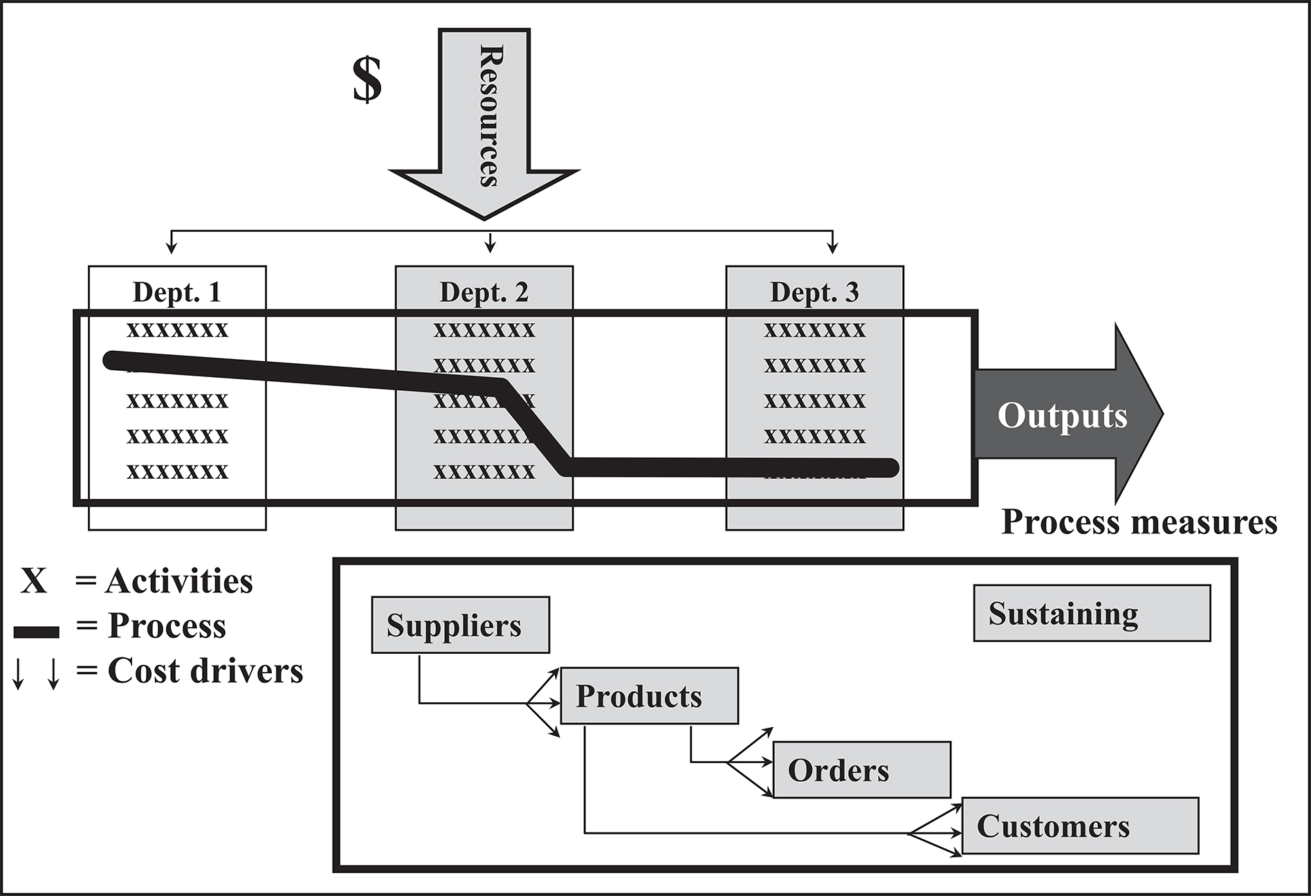
Examine the ABC/M cost assignment network in Figure 6-1, which consists of three modules connected by cost assignment paths. Imagine the cost assignment paths as pipes and straws in which the diameter of each path reflects the amount of cost flowing. The power of an ABC/M model is that the cost assignment paths and their destinations (ie, cost objects) provide traceability to assign costs from beginning to end, from resource expenses to costs for each type of (or each specific) customer—the origin for all costs and expenses.

Figure 6-1: ABC/M Cost Assignment Network

Source: Copyright Gary Cokins. Used with permission.

It may be useful to mentally reverse all the arrowheads in Figure 6-1. This polar switch reveals that all expenses originate with a demand-pull from customers, and the calculated costs simply measure the causal effect. The ABC/M network is basically a snapshot view of the organisation conducted during a specific time period.

Resources, at the top of the cost assignment network in Figure 6-1, are the capacity to perform work because they represent all the available means that work activities can draw on. Resources can be thought of as the organisation’s chequebook because this is where all the period’s expenditure transactions are accumulated and sorted into buckets of spending. Examples of resources are salaries, operating supplies or electrical power. These are the period’s cash outlays and amortised cash outlays, such as for depreciation, from a prior period. It is during this step that the applicable resource drivers are developed as the mechanism to convert resource expenses into activity costs. A popular basis for tracing or assigning resource expenses is the time (eg, number of minutes) that people or equipment are performing activities. An alternative and popular resource driver is the percentage splits of time amongst activities, which is easier and accomplishes a comparable result. Although these proportions are estimated, the estimates are sufficient for adequate cost accuracy of final cost objects.

The activity module is where work is performed by people, equipment and assets. It is where resources are converted into some type of output. The activity cost assignment step contains the structure to assign activity costs to cost objects (or to other activities), utilising activity drivers as the mechanism to accomplish this assignment.

Cost objects, at the bottom of the cost assignment network, represent the broad variety of outputs, services and channels where costs accumulate. The customers are the final-final cost objects. Their existence ultimately creates the need for a cost structure in the first place. Cost objects are the persons or things that benefit from incurring work activities. Examples of cost objects are products, service lines, distribution channels, customers and outputs of internal processes. Cost objects can be thought of as the ‘what’ or ‘for whom’ that work activities are done.

Some activities in an organisation do not directly contribute to customer value, responsiveness and quality. That does not mean those activities can be eliminated or even reduced without doing harm to the business entity. For example, preparing required regulatory reports does not add to the value of any cost object or to the satisfaction of the customer. However, that type of work activity does have value to the organisation because it enables it to function in a legal manner. These types of activity costs are usually traced to a sustaining cost object group popularly called business (or organisational) sustaining costs. This modelling technique separates the business sustaining costs as not being involved with making or delivering a product or serving a customer. It prevents unfairly over-costing products or customers yet allows for all expenses to be traced (and, if needed, reconciled back to the general ledger or source systems (eg, payroll, purchasing). Business sustaining costs are described later in this chapter.

Although some people are initially intimidated by Figure 6-1, it makes more sense the more you work with ABC/M. Also, the ABC/M cost assignment network is related to an observation that has become known as Metcalf’s Law, which states ‘The value of a network increases as the number of nodes increases.’

My conclusion about ABC/M is that the key to a good ABC/M system is the design and architecture of its cost assignment network. It is also the primary determinant of accuracy of final cost objects. (The topic of cost accuracy is later discussed.) The nodes are the sources and destinations through which all the expenses are reassigned into costs. Their configuration helps deliver the utility and value of the data for decision making.

DRIVERS: RESOURCE, COST, ACTIVITY AND COST OBJECT DRIVERS

There is probably no term, other than activity, that has become more identified with ABC/M than the term driver and its several variations. The problem is a driver is used in several ways with varying meanings. To be very clear, a cost driver is something that can be described in words but not necessarily in numbers. For example, a storm would be a cost driver that results in much clean-up work activities and their resulting costs. In contrast, the activity drivers in ABC/M’s cost assignments must be quantitative. They use measures, including percentage splits, that apportion costs to cost objects. In the ABC/M vertical cost assignment view, there are three types of drivers, and all are required to be quantitative:

• Resource drivers trace expenditures (cash outlays, such as salaries) to work activities.

• Activity drivers trace activity costs to cost objects.

• Cost object drivers trace cost object costs to other cost objects.

In the ABC/M vertical cost assignment view, activity drivers will have their own higher order cost drivers, as in the storm example. Cost drivers and activity drivers serve different purposes. Activity drivers are output measures that reflect the usage of each work activity, and they must be quantitatively measurable. An activity driver, which relates a work activity to cost objects, meters out the work activity based on the unique diversity and variation of the cost objects that are consuming the work activity. A cost driver is a driver of a higher order than activity drivers. A storm was the previously mentioned example. One cost driver can affect multiple activities. A cost driver need not be measurable but can simply be described as a triggering event. The term describes the larger scale causal event that influences the frequency, intensity or magnitude of a workload and, therefore, it influences the amount of work done that translates to the cost of the activities.

The third type of driver—a cost object driver—applies to cost objects after all activity costs have already been logically assigned. Note that cost objects can be consumed or used by other cost objects. For example, when a specific customer purchases a mix of products, similar to you placing different items in your grocery cart than another shopper, the quantities purchased are a cost object driver. The source data is typically from the sales or invoicing system.

BUSINESS AND ORGANISATIONAL SUSTAINING COSTS

As previously mentioned, certain types of activity costs trace to business sustaining cost objects, which is similar to other types that trace to product, service line and customer cost objects. The structure of expanded ABC/M systems capitalises on the use of sustaining activities traced to sustaining cost objects to segregate product and customer-related activity costs or to segment product or customer activity costs that cannot be identified as specific to unique products or customers.

Business or infrastructure sustaining costs are those costs not caused by products or customer service needs. The consumption of these costs cannot be logically or causally traced to products, services, customers or service recipients. One example is the closing of the books each month by the accounting department. How can one measure which product caused more or less of that work? One cannot.

Another example is a green lawn. Which customers or products cause the grass to grow? These kinds of activity cost cannot be directly charged to a customer, product or service in any fair and equitable way. There is simply no ‘use-based’ causality originating from the product or customer. (Yet, overhead expenses are routinely and unfairly allocated this way despite the result being flawed and misleading costs.) Recovering these costs through pricing or funding may eventually be required, but that is a different issue. The issue here is fairly charging cost objects when no causal relationship exists and preventing overstating their costs.

Business-sustaining costs (or organisation-sustaining costs for governments and not-for-profit organisations) can eventually be fully absorbed into products or customers, but such a cost allocation is blatantly arbitrary. There simply is no cause and effect relationship between a business-sustaining cost object and the other final cost objects. If and when these costs are assigned to final cost objects, organisations that do so often refer to them as a management tax, representing a cost of doing business apart from the products and service lines. If forced to fully absorb sustaining costs, the only fair way is to first assign and calculate all other cost objects and then use those cost results as the assignment basis. Like a rising tide lifts all boats, all cost objects are equitably charged with the tax.

Examples of final cost objects that comprise business-sustaining cost objects include senior management (at individual levels, such as headquarters, corporate, division and local) or government regulatory agencies (such as environmental, occupational safety or tax authorities). In effect, regulatory organisations (through their policies and compliance requirements) or executives (through their informal desires such as briefings or forecasts) place demands on work activities not caused by, or attributable to, specific products or customers.

Other categories of expenses that may be included as business-sustaining costs are idle, but available, capacity costs or research and development (R&D). R&D expenses might be optionally assigned into the business-sustaining costs so that the timing of the recognition of expenses is reasonably matched with turnover recognition for sales of the products or service lines. Because activity-based costing is management accounting, not regulated financial reporting, strict rules of generally accepted accounting principles do not need to be followed, however, they can be borrowed.

THE TWO VIEWS OF COSTS: THE ASSIGNMENT VIEW VERSUS THE PROCESS VIEW

Substantial confusion exists between the costs of processes and output costing (eg, product costs), even by accountants. Let’s clarify the differences.

As earlier mentioned, ABC/M requires two separate cost assignment structures: (1) the horizontal process cost scheme governed by the time sequence of activities that belong to the various processes, and (2) the vertical cost re-assignment scheme governed by the variation and diversity of the cost objects. In effect, think of this vertical ABC/M cost assignment view as being time-blind. The ABC/M process costing view, at the activity stage, is blind to output mix. The cost assignment and business process costing are two different views of the same resource expenses and their activity costs. They are equivalent in amount, but the display of the information is radically different in each view.

Vertical Axis

The vertical axis, as illustrated in Figure 6-2, reflects costs that are sensitive to demands from all forms of product, channel and customer diversity and variety. The work activities consume the resources, and the products and customer services consume the work activities. The ABC/M cost assignment view is a cost-consumption chain. When each cost is traced based on its unique quantity or proportion of its driver, all the resource expenses are eventually re-aggregated into the final cost objects. This method provides much more accurate measures of product, channel and customer costs than the traditional and arbitrary, broadly averaged cost allocation method without causality.

Figure 6-2: The Vertical View of Assigning Costs

Source: Copyright Gary Cokins. Used with permission.

Horizontal Axis

The horizontal view, as illustrated in Figure 6-3, of activity costs represents the business process view. A business process can be defined as two or more activities, or a network of activities, with a common purpose. Activity costs belong to the business processes. Across each process, the activity costs are sequential and additive. In this orientation, activity costs satisfy the requirements for popular flow-charting (eg, swim lane diagrams) and process mapping and modelling techniques. Business process-based thinking can be visualised as tipping the organisation chart 90 degrees. ABC/M provides the activity cost elements for process costing that are not available from the general ledger.

Figure 6-3: The Horizontal View of Sequencing Costs

Source: Copyright Gary Cokins. Used with permission.

In summary, the vertical cost assignment view explains what specific things cost using their resource and activity drivers, whereas the horizontal process view illustrates how much processes cost.

HOW DOES ACTIVITY-BASED COSTING COMPUTE BETTER ACCURACIES?

When people who are first exposed to ABC/M hear the phrase, ‘It is better to be approximately correct than precisely inaccurate,’ they smile because they know exactly what that means in their organisation. However they usually do not know what causes ABC/M to produce substantially better accuracy relative to their existing legacy costing system despite ABC/M’s abundant use of estimates and approximations. One of the explanations, which is counter-intuitive to many, is that the initial errors from resource driver estimates in an ABC/M assignment system cancel out. This is due, in part, because allocating (ie, re-assigning expenses into costs) is a closed system with a zero sum total error in the total costs of the final cost objects. Every assignment normalises to 100%, and any errors offset and cancel out. This is ABC/M’s activity cost error dampening effect.

The starting amount of expenses to be traced and assigned can be assumed to be 100.000% accurate because they come from the general ledger accounting system (or source payroll and purchasing data sources) that is specially designed to accumulate and summarise the detailed spending transactions. However, subsequently, as we re-assign expenses into calculated costs, imprecise inputs do not automatically result in inaccurate outputs. That is, precision is not synonymous with accuracy. On the surface this is counter-intuitive. In ABC/M’s cost assignment view, estimating error does not compound, it dampens out. These are properties of statistics found in equilibrium networks (ie, the amount of expenses and costs remains constant through the cost flow network), and ABC/M is a cost re-assignment network much more than it is an accounting system.

Even more startling is that the cost assignment network structure itself is an even greater determinant that influences accuracy because each assignment path is detecting only the cost objects for which a consumption relationship exits. Compare that with broadly averaged cost allocations that disproportionately charge every cost object. (Remember the example of splitting the bill at the restaurant in the previous chapter?) The lesson is that costing is modelling.

In ABC/M, poor model design leads to poor results. A well-known and painful lesson about activity-based costing is that when an ABC/M system implementation system falls short of its expectations, it is often because the system was over-engineered in size and detail. The ABC/M system usually quickly reached diminishing returns in extra accuracy for incremental levels of effort, but this effect was not recognised by the ABC/M project team. The system was built so large in size that the administrative effort to collect the data and maintain the system was ultimately judged to be not worth the perceived benefits. This results in a ‘death by details’ ABC/M project. It is unsustainable. In short, over-designed ABC/M systems are too detailed relative to their intended use.

As the designers construct their ABC/M information system, they usually suffer from a terrible case of lack of depth perception. There is no perspective from which they can judge how high or low or summarised or detailed they are. The implementation of an ABC/M system is usually influenced by accountants, and an accountant’s natural instincts include a ‘lowest common denominator mentality.’ Accountants usually assume a detailed and comprehensive level of data collection based on the premise that if you collect a great amount of detail everywhere, from everybody, and about everything they do, you can then summarise anywhere. This is a ‘just in case’ approach in anticipation of any future, remote questions. The term accuracy requirements is apparently not in many accountants’ vocabulary. As a result, their ABC/M models tend to become excessively large. They may ultimately become unmaintainable and not sustainable. Eventually the ABC/M system does not appear to be worth the effort. I am not criticising or attacking accountants. Years of training reinforce their high need for precision. However, ABC/M requires a bias towards practical use of the data.

The illusion that more detailed and granular data provide higher accuracy is part of the explanation for this behaviour. Another explanation for oversized ABC/M models is that at the outset of an ABC/M project, it is nearly impossible to pre-determine what levels of detail to go to. There are so many interdependencies in an ABC/M model that, as a result, it presents a problem. It is almost impossible to perform one of the earlier steps of a traditional IT function’s systems development project plan—defining data requirements.

As an example, a question frequently asked by organisations implementing activity-based costing is, ‘How many activities should be included in an activity-based costing system?’ There is no correct answer because the number of activities is dependent on the answer to several other questions, such as, ‘What problem are you trying to solve with the activity-based costing data?’ In other words, the size, depth, granularity and accuracy of an activity-based costing system are dependent variables determined by other factors. The level of detail and accuracy of an activity-based costing system depends on what decisions the data will be used for. Implementing an ABC/M system with rapid prototyping, a technique that quickly resolves this problem, is discussed later in this chapter.

What is missing in most ABC/M implementations is a good understanding of what factors actually determine the accuracy of the ABC/M-calculated outputs. That is, what are the major determinants of higher accuracy of final cost objects? The following assertion will likely be counter-intuitive, not only to accountants, but also to everyone who designs and builds ABC/M systems. As earlier mentioned, ABC/M’s substantially improved accuracy relative to traditional approaches actually resides more in the ABC/M cost assignment network structure itself than in the activity costs and the activity driver quantities. That is, the reason that the products, service lines, channels and customer costs are so reasonably accurate has less to do with their driver input data than with the architecture of the cost flow paths that make up the ABC/M cost assignment network.

Achieving success with ABC/M initially begins with overcoming the ABC/M levelling problem—right-sizing the model to a proper level of detail and disaggregation. Once the appropriate levels are stabilised at a Goldilocks level (ie, not too detailed nor too summarised), then the connection of the ABC/M data to business problems, their analysis and ultimate solutions can follow. In the end, the payback from implementing ABC/M can be accelerated.

ACTIVITY-BASED MANAGEMENT RAPID PROTOTYPING: GETTING QUICK AND ACCURATE RESULTS

The ABC/M levelling problem can be partly solved using the increasingly popular technique of ABC/M rapid prototyping. This is a method of building the first ABC/M model in a few short days, relying on knowledgeable employees, followed by a few weeks of iterative re-modelling to gradually, but not excessively, scale up the size of the model. Its benefits are accelerated learning and right-sizing the ABC/M model. In addition to this highly managed trial and error approach, effective levelling of the ABC/M model can be achieved through better thinking. Figure 6-4 illustrates ABC/M iterative re-modelling.

Figure 6-4: Rapid Prototyping with Iterative Remodelling.

Each iteration enhances the use of the ABC/M system.

Source: Copyright Gary Cokins. Used with permission.

In a closed cost assignment system, there is a zero sum error, and error dampens out into cost objects. Figure 6-5 shows several asymptotic curves that all have the same ultimate destination: perfectly accurate costs of cost objects (especially final cost objects), in which the accuracy level is represented by the vertical axis. The horizontal axis represents the level of administrative effort to collect, calculate and report the data. As previously explained, for each incremental level of effort to collect more and better data, there is proportionately less improvement in accuracy. The asymptotic curves reflect both the error-dampening effect of offsetting activity cost error and improved design of the cost assignment network structure.

Figure 6-5: Balancing Levels of Accuracy With Effort

Source: Copyright Gary Cokins. Used with permission.

The question ‘Is the climb worth the view?’ is applicable to ABC/M. That is, by building a more detailed and slightly more accurate ABC/M model, will the answer to your question be better answered? Avoid the creeping elegance syndrome, ie the tendency to add details at the expense of the basic design. Larger models introduce maintenance issues. ABC/M rapid prototyping accelerates a team’s understanding and acceptance of ABC/M by quickly giving them a vision of what their completed ABC/M system will look like—once scaled to its proper level of detail—and how they will use the new ABC/M information.

PRODUCT PROFITABILITY ANALYSIS

Because the product costs from ABC/M will be different compared to the costs from the existing, broadly-averaged and non-causal relationship method, and the selling prices are unaffected, product profits will also be different. They have to be different. It is simple math. The top line sales minus the middle line costs equals profit. Profit is a derivative of the first two lines in the equation.

Because analysis is expanding beyond product standard service line profitability to include channels and customers, the next chapter will discuss all the profit contribution layers.

TWO ALTERNATIVE EQUATIONS FOR COSTING ACTIVITIES AND COST OBJECTS

Two alternative approaches exist for computing activity costs and the costs of cost objects, such as products. The two approaches differ based on which data one prefers to collect versus calculate and how your organisation prefers to use feedback data to control its costs. The two approaches are as follows:

• Activity driver equations. First, activity costs are derived (via surveys, timesheets, estimates, etc). Then the quantity, frequency or intensity of the activity driver is collected per each activity. A unit cost rate per each activity driver is computed and then applied to all the cost objects based on their unique quantity of the activity driver events (eg, number of invoices processed). This is re-calculated for each time period for each work activity.

• Cost object equations. This approach begins with an in-depth time measurement study of work tasks and processes. It is the basis for time-driven ABC. In the study, the per unit time element for various (and optional) processing steps for each product (or product group) and each type of order are surveyed with deep time studies. Then each product and type of order is profiled with an equation specifying the sum of the number of transactions (eg, events) for each product or type of order. Finally, the quantity of the products and order types is counted for the period and backflushed against each product’s or order’s standard minutes-per-event to calculate an activity cost. This activity cost assumes the standard rate and is not the actual activity costs. The premise that this assumption is acceptable is that micro-measured activities do not vary much over time. What drives requirements for expenses is the varying mix and volume of products and type of orders.

Both approaches are intended to compute profitability margins for products, order types and, ideally, for channels and customer types as well. Each approach arrives at comparable answers in different ways. With regard to operational control and feedback, the two approaches are different because of which data each approach collects and computes. The activity driver equation approach monitors trends in activity driver cost rates, and it can be used to calculate and report cost variances to monitor efficiencies. It consequently focuses on activity performance. In contrast, the cost object equation approach attempts to provide information about the magnitude of idle capacity (primarily number of employees), so this approach focuses more on usage levels of resources and less on activity performance.

Figure 6-6 displays where these two approaches are located with respect to the ABC/M cost assignment network and how they differ. The activity driver equation approach solves for cost of the cost objects based on measuring or estimating activity costs and tracing them per events (ie, activity driver quantities). In contrast, the cost object equation approach begins with product and order type profiles, collects volume and mix data, and then solves for the activity costs, assuming the standard times are correct and incurred. It starts with a low level of characteristics of the cost object. This approach appears to reverse-calculate to determine the activity costs.

Figure 6-6: Two Cost Equation Approaches.

Source: Copyright Gary Cokins. Used with permission.

In practice, for historical reporting, there is no proper direction of flow of costs. Costing is modelling, and historical costs are like an electric circuit—it is a directionless transformation of expenses into costs. So both of these equation-based costing methods are in synchronisation. They simply arrive at a similar answer using different assumptions. (However, for predictive costing, which is a separate topic, direction of flow is from outputs placing demands on work that then draw on resource capacity. Predictive costing uses historical ABC/M as its foundation but includes many more assumptions.)

For the activity driver equation approach, you solve for the activity driver rate by assuming that data for the other two factors can be collected or reasonably estimated. For the cost object equation approach, you solve for the activity cost, at a standard cost, by presuming that processing times for each product’s (ie, output) characteristics have been measured, profiles for each product configured, and then the product mix volumes are reported. The superior ABC/M software can compute costs in both directions.

Regardless of which equation-based approach is used, be cautious to first recognise the primary reasons you may be pursuing ABC/M data. Then, presuming there will be some interest in using the ABC/M for operational cost control and feedback, be clear in what type of feedback costs you will be more interested.