
Chapter 3. Streaming Architectures
The implementation of a distributed data analytics system has to deal with the management of a pool of computational resources, as in-house clusters of machines or reserved cloud-based capacity, to satisfy the computational needs of a division or even an entire company. Since teams and projects rarely have the same needs over time, clusters of computers are best amortized if they are a shared resource among a few teams, which requires dealing with the problem of multitenancy.
When the needs of two teams differ, it becomes important to give each a fair and secure access to the resources for the cluster, while making sure the computing resources are best utilized over time.
This need has forced people using large clusters to address this heterogeneity with modularity, making several functional blocks emerge as interchangeable pieces of a data platform. For example, when we refer to database storage as the functional block, the most common component that delivers that functionality is a relational database such as PostgreSQL or MySQL, but when the streaming application needs to write data at a very high throughput, a scalable column-oriented database like Apache Cassandra would be a much better choice.
In this chapter, we briefly explore the different parts that comprise the architecture of a streaming data platform and see the position of a processing engine relative to the other components needed for a complete solution. After we have a good view of the different elements in a streaming architecture, we explore two architectural styles used to approach streaming applications: the Lambda and the Kappa architectures.
Components of a Data Platform
We can see a data platform as a composition of standard components that are expected to be useful to most stakeholders and specialized systems that serve a purpose specific to the challenges that the business wants to address.
Figure 3-1 illustrates the pieces of this puzzle.

Figure 3-1. The parts of a data platform
Going from the bare-metal level at the bottom of the schema to the actual data processing demanded by a business requirement, you could find the following:
- The hardware level
-
On-premises hardware installations, datacenters, or potentially virtualized in homogeneous cloud solutions (such as the T-shirt size offerings of Amazon, Google, or Microsoft), with a base operating system installed.
- The persistence level
-
On top of that baseline infrastructure, it is often expected that machines offer a shared interface to a persistence solution to store the results of their computation as well as perhaps its input. At this level, you would find distributed storage solutions like the Hadoop Distributed File System (HDFS)—among many other distributed storage systems. On the cloud, this persistence layer is provided by a dedicated service such as Amazon Simple Storage Service (Amazon S3) or Google Cloud Storage.
- The resource manager
-
After persistence, most cluster architectures offer a single point of negotiation to submit jobs to be executed on the cluster. This is the task of the resource manager, like YARN and Mesos, and the more evolved schedulers of the cloud-native era, like Kubernetes.
- The execution engine
-
At an even higher level, there is the execution engine, which is tasked with executing the actual computation. Its defining characteristic is that it holds the interface with the programmer’s input and describes the data manipulation. Apache Spark, Apache Flink, or MapReduce would be examples of this.
- A data ingestion component
-
Besides the execution engine, you could find a data ingestion server that could be plugged directly into that engine. Indeed, the old practice of reading data from a distributed filesystem is often supplemented or even replaced by another data source that can be queried in real time. The realm of messaging systems or log processing engines such as Apache Kafka is set at this level.
- A processed data sink
-
On the output side of an execution engine, you will frequently find a high-level data sink, which might be either another analytics system (in the case of an execution engine tasked with an Extract, Transform and Load [ETL] job), a NoSQL database, or some other service.
- A visualization layer
-
We should note that because the results of data-processing are useful only if they are integrated in a larger framework, those results are often plugged into a visualization. Nowadays, since the data being analyzed evolves quickly, that visualization has moved away from the old static report toward more real-time visual interfaces, often using some web-based technology.
In this architecture, Spark, as a computing engine, focuses on providing data processing capabilities and relies on having functional interfaces with the other blocks of the picture. In particular, it implements a cluster abstraction layer that lets it interface with YARN, Mesos, and Kubernetes as resource managers, provides connectors to many data sources while new ones are easily added through an easy-to-extend API, and integrates with output data sinks to present results to upstream systems.
Architectural Models
Now we turn our attention to the link between stream processing and batch processing in a concrete architecture. In particular, we’re going to ask ourselves the question of whether batch processing is still relevant if we have a system that can do stream processing, and if so, why?
In this chapter, we contrast two conceptions of streaming application architecture: the Lambda architecture, which suggests duplicating a streaming application with a batch counterpart running in parallel to obtain complementary results, and the Kappa architecture, which purports that if two versions of an application need to be compared, those should both be streaming applications. We are going to see in detail what those architectures intend to achieve, and we examine that although the Kappa architecture is easier and lighter to implement in general, there might be cases for which a Lambda architecture is still needed, and why.
The Use of a Batch-Processing Component in a Streaming Application
Often, if we develop a batch application that runs on a periodic interval into a streaming application, we are provided with batch datasets already—and a batch program representing this periodic analysis, as well. In this evolution use case, as described in the prior chapters, we want to evolve to a streaming application to reap the benefits of a lighter, simpler application that gives faster results.
In a greenfield application, we might also be interested in creating a reference batch dataset: most data engineers don’t work on merely solving a problem once, but revisit their solution, and continuously improve it, especially if value or revenue is tied to the performance of their solution. For this purpose, a batch dataset has the advantage of setting a benchmark: after it’s collected, it does not change anymore and can be used as a “test set.” We can indeed replay a batch dataset to a streaming system to compare its performance to prior iterations or to a known benchmark.
In this context, we identify three levels of interaction between the batch and the stream-processing components, from the least to the most mixed with batch processing:
- Code reuse
-
Often born out of a reference batch implementation, seeks to reemploy as much of it as possible, so as not to duplicate efforts. This is an area in which Spark shines, since it is particularly easy to call functions that transform Resilient Distributed Databases (RDDs) and DataFrames—they share most of the same APIs, and only the setup of the data input and output is distinct.
- Data reuse
-
Wherein a streaming application feeds itself from a feature or data source prepared, at regular intervals, from a batch processing job. This is a frequent pattern: for example, some international applications must handle time conversions, and a frequent pitfall is that daylight saving rules change on a more frequent basis than expected. In this case, it is good to be thinking of this data as a new dependent source that our streaming application feeds itself off.
- Mixed processing
-
Wherein the application itself is understood to have both a batch and a streaming component during its lifetime. This pattern does happen relatively frequently, out of a will to manage both the precision of insights provided by an application, and as a way to deal with the versioning and the evolution of the application itself.
The first two uses are uses of convenience, but the last one introduces a new notion: using a batch dataset as a benchmark. In the next subsections, we see how this affects the architecture of a streaming application.
Referential Streaming Architectures
In the world of replay-ability and performance analysis over time, there are two historical but conflicting recommendations. Our main concern is about how to measure and test the performance of a streaming application. When we do so, there are two things that can change in our setup: the nature of our model (as a result of our attempt at improving it) and the data that the model operates on (as a result of organic change). For instance, if we are processing data from weather sensors, we can expect a seasonal pattern of change in the data.
To ensure we compare apples to apples, we have already established that replaying a batch dataset to two versions of our streaming application is useful: it lets us make sure that we are not seeing a change in performance that is really reflecting a change in the data. Ideally, in this case, we would test our improvements in yearly data, making sure we’re not overoptimizing for the current season at the detriment of performance six months after.
However, we want to contend that a comparison with a batch analysis is necessary, as well, beyond the use of a benchmark dataset—and this is where the architecture comparison helps.
The Lambda Architecture
The Lambda architecture (Figure 3-2) suggests taking a batch analysis performed on a periodic basis—say, nightly—and to supplement the model thus created with streaming refinements as data comes, until we are able to produce a new version of the batch analysis based on the entire day’s data.
It was introduced as such by Nathan Marz in a blog post, “How to beat the CAP Theorem”.1 It proceeds from the idea that we want to emphasize two novel points beyond the precision of the data analysis:
-
The historical replay-ability of data analysis is important
-
The availability of results proceeding from fresh data is also a very important point
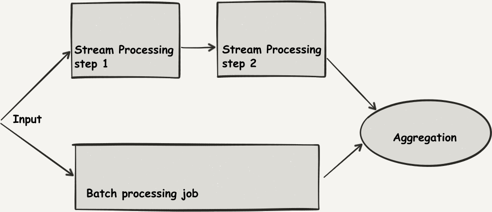
Figure 3-2. The Lambda architecture
This is a useful architecture, but its drawbacks seem obvious, as well: such a setup is complex and requires maintaining two versions of the same code, for the same purpose. Even if Spark helps in letting us reuse most of our code between the batch and streaming versions of our application, the two versions of the application are distinct in life cycles, which might seem complicated.
An alternative view on this problem suggests that it would be enough to keep the ability to feed the same dataset to two versions of a streaming application (the new, improved experiment, and the older, stable workhorse), helping with the maintainability of our solution.
The Kappa Architecture
This architecture, as outlined in Figure 3-3, compares two streaming applications and does away with any batching, noting that if reading a batch file is needed, a simple component can replay the contents of this file, record by record, as a streaming data source. This simplicity is still a great benefit, since even the code that consists in feeding data to the two versions of this application can be reused. In this paradigm, called the Kappa architecture ([Kreps2014]), there is no deduplication and the mental model is simpler.

Figure 3-3. The Kappa architecture
This begs the question: is batch computation still relevant? Should we convert our applications to be all streaming, all the time?
We think some concepts stemming from the Lambda architecture are still relevant; in fact, they’re vitally useful in some cases, although those are not always easy to figure out.
There are some use cases for which it is still useful to go through the effort of implementing a batch version of our analysis and then compare it to our streaming solution.
Streaming Versus Batch Algorithms
There are two important considerations that we need to take into account when selecting a general architectural model for our streaming application:
-
Streaming algorithms are sometimes completely different in nature
-
Streaming algorithms can’t be guaranteed to measure well against batch algorithms
Let’s explore these thoughts in the next two sections using motivating examples.
Streaming Algorithms Are Sometimes Completely Different in Nature
Sometimes, it is difficult to deduce batch from streaming, or the reverse, and those two classes of algorithms have different characteristics. This means that at first glance we might not be able to reuse code between both approaches, but also, and more important, that relating the performance characteristics of those two modes of processing should be done with high care.
To make things more precise, let’s look at an example: the buy or rent problem. In this case, we decide to go skiing. We can buy skis for $500 or rent them for $50. Should we rent or buy?
Our intuitive strategy is to first rent, to see if we like skiing. But suppose we do: in this case, we will eventually realize we will have spent more money than we would have if we had bought the skis in the first place.
In the batch version of this computation, we proceed “in hindsight,” being given the total number of times we will go skiing in a lifetime. In the streaming, or online version of this problem, we are asked to make a decision (produce an output) on each discrete skiing event, as it happens. The strategy is fundamentally different.
In this case, we can consider the competitive ratio of a streaming algorithm. We run the algorithm on the worst possible input, and then compare its “cost” to the decision that a batch algorithm would have taken, “in hindsight.”
In our buy-or-rent problem, let’s consider the following streaming strategy: we rent until renting makes our total spending as much as buying, in which case we buy.
If we go skiing nine times or fewer, we are optimal, because we spend as much as what we would have in hindsight. The competitive ratio is one. If we go skiing 10 times or more, we pay $450 + $500 = $950. The worst input is to receive 10 “ski trip” decision events, in which case the batch algorithm, in hindsight, would have paid $500. The competitive ratio of this strategy is (2 – 1/10).
If we were to choose another algorithm, say “always buy on the first occasion,” then the worst possible input is to go skiing only once, which means that the competitive ratio is $500 / $50 = 10.
Note
The performance ratio or competitive ratio is a measure of how far from the optimal the values returned by an algorithm are, given a measure of optimality. An algorithm is formally ρ-competitive if its objective value is no more than ρ times the optimal offline value for all instances.
A better competitive ratio is smaller, whereas a competitive ratio above one shows that the streaming algorithm performs measurably worse on some inputs. It is easy to see that with the worst input condition, the batch algorithm, which proceeds in hindsight with strictly more information, is always expected to perform better (the competitive ratio of any streaming algorithm is greater than one).
Streaming Algorithms Can’t Be Guaranteed to Measure Well Against Batch Algorithms
Another example of those unruly cases is the bin-packing problem. In the bin-packing problem, an input of a set of objects of different sizes or different weights must be fitted into a number of bins or containers, each of them having a set volume or set capacity in terms of weight or size. The challenge is to find an assignment of objects into bins that minimizes the number of containers used.
In computational complexity theory, the offline ration of that algorithm is known to be NP-hard. The simple variant of the problem is the decision question: knowing whether that set of objects will fit into a specified number of bins. It is itself NP-complete, meaning (for our purposes here) computationally very difficult in and of itself.
In practice, this algorithm is used very frequently, from the shipment of actual goods in containers, to the way operating systems match memory allocation requests, to blocks of free memory of various sizes.
There are many variations of these problems, but we want to focus on the distinction between online versions—for which the algorithm has as input a stream of objects—and offline versions—for which the algorithm can examine the entire set of input objects before it even starts the computing process.
The online algorithm processes the items in arbitrary order and then places each item in the first bin that can accommodate it, and if no such bin exists, it opens a new bin and puts the item within that new bin. This greedy approximation algorithm always allows placing the input objects into a set number of bins that is, at worst, suboptimal; meaning we might use more bins than necessary.
A better algorithm, which is still relatively intuitive to understand, is the first fit decreasing strategy, which operates by first sorting the items to be inserted in decreasing order of their sizes, and then inserting each item into the first bin in the list with sufficient remaining space. That algorithm was proven in 2007 to be much closer to the optimal algorithm producing the absolute minimum number of bins ([Dosa2007]).
The first fit decreasing strategy, however, relies on the idea that we can first sort the items in decreasing order of sizes before we begin processing them and packing them into bins.
Now, attempting to apply such a method in the case of the online bin-packing problem, the situation is completely different in that we are dealing with a stream of elements for which sorting is not possible. Intuitively, it is thus easy to understand that the online bin-packing problem—which by its nature lacks foresight when it operates—is much more difficult than the offline bin-packing problem.
Warning
That intuition is in fact supported by proof if we consider the competitive ratio of streaming algorithms. This is the ratio of resources consumed by the online algorithm to those used by an online optimal algorithm delivering the minimal number of bins by which the input set of objects encountered so far can be packed. This competitive ratio for the knapsack (or bin-packing) problem is in fact arbitrarily bad (that is, large; see [Sharp2007]), meaning that it is always possible to encounter a “bad” sequence in which the performance of the online algorithm will be arbitrarily far from that of the optimal algorithm.
The larger issue presented in this section is that there is no guarantee that a streaming algorithm will perform better than a batch algorithm, because those algorithms must function without foresight. In particular, some online algorithms, including the knapsack problem, have been proven to have an arbitrarily large performance ratio when compared to their offline algorithms.
What this means, to use an analogy, is that we have one worker that receives the data as batch, as if it were all in a storage room from the beginning, and the other worker receiving the data in a streaming fashion, as if it were on a conveyor belt, then no matter how clever our streaming worker is, there is always a way to place items on the conveyor belt in such a pathological way that he will finish his task with an arbitrarily worse result than the batch worker.
The takeaway message from this discussion is twofold:
Summary
In conclusion, the news of batch processing’s demise is overrated: batch processing is still relevant, at least to provide a baseline of performance for a streaming problem. Any responsible engineer should have a good idea of the performance of a batch algorithm operating “in hindsight” on the same input as their streaming application:
-
If there is a known competitive ratio for the streaming algorithm at hand, and the resulting performance is acceptable, running just the stream processing might be enough.
-
If there is no known competitive ratio between the implemented stream processing and a batch version, running a batch computation on a regular basis is a valuable benchmark to which to hold one’s application.
1 We invite you to consult the original article if you want to know more about the link with the CAP theorem (also called Brewer’s theorem). The idea was that it concentrated some limitations fundamental to distributed computing described by the theorem to a limited part of the data-processing system. In our case, we’re focusing on the practical implications of that constraint.