CHAPTER 30
Interest Rate Options
Amir Sadr
Given an underlying asset, derivatives or contingent claims are contracts with specified payoffs based on the value of the underlying. The simplest contingent claim—after a forward contract—is a European Style exercise option which has a specified payoff at a single exercise time ![]() in the future. For example, a call,
in the future. For example, a call, ![]() , with strike
, with strike ![]() on an asset
on an asset ![]() has the following payoff:
has the following payoff: ![]() , while a put,
, while a put, ![]() , has payoff
, has payoff ![]() . While the value of the contingent claim is known at expiration, the goal of Contingent‐Claim Pricing is to determine its value prior to expiry.
. While the value of the contingent claim is known at expiration, the goal of Contingent‐Claim Pricing is to determine its value prior to expiry.
The Black‐Scholes‐Metron formula was a pioneering result in calculating the price of European‐style options. While their methodology used advanced mathematical techniques to come up with the formula, it was shown later by Cox‐Ross‐Rubenstein (CRR), that the same formula can be obtained and understood using much simpler techniques. This new methodology goes under the name of Risk‐Neutral Valuation and is the modern framework for contingent claim valuation. Its basic result is that any contingent claim's value is its expected discounted value of its cash‐flows in a risk‐neutral world. We explain this by using the most basic model: A 1‐step binomial model. It is often said (and is indeed true) that all you need to understand option pricing is to fully understand the 1‐step binomial model. We shall spend some time to fully explore this simple yet powerful model.
1‐STEP BINOMIAL MODEL
Given today's ![]() price of an underlying asset
price of an underlying asset ![]() , consider a European‐style contingent claim
, consider a European‐style contingent claim ![]() with a single expiration time
with a single expiration time ![]() in the future. Assume that the underlying asset has no cash‐flows over the period
in the future. Assume that the underlying asset has no cash‐flows over the period ![]() , and let us consider the simplest case where the underlying asset at expiration can only take on two values,
, and let us consider the simplest case where the underlying asset at expiration can only take on two values, ![]() ,
, ![]() , as shown in Figure 30.1. Let
, as shown in Figure 30.1. Let ![]() and
and ![]() denote the corresponding then‐known values of the contingent claim in each state at expiration.
denote the corresponding then‐known values of the contingent claim in each state at expiration.

Figure 30.1: A 1‐step binomial model
Our goal is to construct a portfolio today (![]() ) so that its value at expiration,
) so that its value at expiration, ![]() , replicates the value of the contingent claim. Therefore if we are the seller of the option, we can replicate the option's contingent cash‐flows at expiration via this replicating portfolio. The fair price of the option today,
, replicates the value of the contingent claim. Therefore if we are the seller of the option, we can replicate the option's contingent cash‐flows at expiration via this replicating portfolio. The fair price of the option today, ![]() , would be the cost of setting up the portfolio.
, would be the cost of setting up the portfolio.
Our portfolio consists of taking a position in the asset, ![]() units of it, by financing it via a risk‐free loan of size
units of it, by financing it via a risk‐free loan of size ![]() at the prevalent risk‐free rate
at the prevalent risk‐free rate ![]() until expiration date
until expiration date ![]() , so the value of the loan at expiration would be
, so the value of the loan at expiration would be ![]() regardless of the state of the world.
regardless of the state of the world.
At expiry, ![]() , if we are in
, if we are in ![]() state of the world, we want this portfolio to be worth
state of the world, we want this portfolio to be worth ![]() :
:
Similarly, if we are in ![]() state of the world, we want the portfolio to be worth
state of the world, we want the portfolio to be worth ![]() :
:
We have two equations and two unknowns (![]() ,
, ![]() ). Solving for these, we get:
). Solving for these, we get:

Therefore, today's value of the contingent claim is:

The seller of the option can charge ![]() as above, take a loan of size
as above, take a loan of size ![]() as above, and use these proceeds to buy
as above, and use these proceeds to buy ![]() units of the asset at spot price
units of the asset at spot price ![]() . At expiration, in either state of the world,
. At expiration, in either state of the world, ![]() or
or ![]() , the value of his holdings (
, the value of his holdings (![]() units of the asset) exactly offsets his liabilities: Repayment of loan plus interest, and cash‐settlement value of the option (
units of the asset) exactly offsets his liabilities: Repayment of loan plus interest, and cash‐settlement value of the option (![]() or
or ![]() ).
).
Note that in the above setup, we did not have to consider the probability of either state happening: as long as ![]() can happen and are the only two possibilities, we are golden!
can happen and are the only two possibilities, we are golden!
However, there are restrictions on the assumed future states. A bit of algebra allows us to rewrite the formula for ![]() as an expected value:
as an expected value:
where

No Arbitrage
Lack of arbitrage is equivalent to ![]() being a probability,
being a probability,
which is equivalent to the following restriction on assumed states:
since for an asset with no interim cash‐flows, ![]() .
.
To see this, consider the case ![]() , which means that the forward is higher than either state in the future:
, which means that the forward is higher than either state in the future: ![]() . In this case, we can sell the asset forward for
. In this case, we can sell the asset forward for ![]() , and deliver it at
, and deliver it at ![]() by buying it at either
by buying it at either ![]() or
or ![]() . Regardless, we have made money with no risk!
. Regardless, we have made money with no risk!
Similarly, if ![]() , then
, then ![]() , and we can ensure a risk‐less profit by buying the asset forward for
, and we can ensure a risk‐less profit by buying the asset forward for ![]() , and selling it higher at expiration at
, and selling it higher at expiration at ![]() or
or ![]() .
.
Therefore, if there is no arbitrage in the above simple economy, ![]() can be considered as a probability, and today's value of the option is simply the expected discounted value of the option payoff under this probability.
can be considered as a probability, and today's value of the option is simply the expected discounted value of the option payoff under this probability.
Risk‐Neutrality
We obtained ![]() by constructing a portfolio that replicates the option payoff, regardless of the probability of each state. We then showed that we can get the same value by taking the expected value under a probability
by constructing a portfolio that replicates the option payoff, regardless of the probability of each state. We then showed that we can get the same value by taking the expected value under a probability ![]() . Other than a mathematical identity—
. Other than a mathematical identity—![]() is the probability that gets you the correct option value, as long as you know the option value!—is there another way of interpreting
is the probability that gets you the correct option value, as long as you know the option value!—is there another way of interpreting ![]() ? The answer is in the affirmative:
? The answer is in the affirmative: ![]() is the probability that a risk‐neutral investor would apply to the above setting.
is the probability that a risk‐neutral investor would apply to the above setting.
Most people are risk‐averse: between a guaranteed return and a risky investment with identical expected returns, they would opt for the former. That is why risky investments (stocks, real‐estate,…) need to have a higher than average expected returns. Otherwise, one could simply put one's money in the bank and have the same return with no volatility.
On the other hand, most of us have bought a lottery ticket or played in casinos, investments whose expected gain is less than what we paid for. These types of investing are examples of risk‐taking, where although risky, we are batting for the fences.
In between, there is an investment behavior that considers any investments with the same expected return as equivalent, and does not require a risk premium for risky bets. Consider such an investor given a choice between 2 investments: 1) Invest ![]() at the bank, and get
at the bank, and get ![]() at
at ![]() , or 2) Buy an asset at
, or 2) Buy an asset at ![]() and either get
and either get ![]() or
or ![]() at
at ![]() . For a risk‐neutral investor, these two investments would be equivalent if
. For a risk‐neutral investor, these two investments would be equivalent if
or equivalently, when

Therefore, rather than setting up a replicating portfolio and computing its value today, we can simply take the expected discounted value of the option payoff using risk‐neutral probabilities.
FROM 1 TIME‐STEP TO 2 TO …
The 2‐state setup is obviously too simplistic. Assets can take a variety of values at expiration. However, using the above setup as a building block, we can arrive at more complex cases. The trick is to subdivide the time from now till expiration into multiple intervals, and for each state in each interval, generate two new arbitrage‐free (bracketing the forward) future states. With enough subdivisions, we can arrive at a richer and more real‐life terminal distribution for the asset.

Figure 30.2: Example of bond option pricing in a 2‐period setting
Consider a 2 time‐step example shown in Figure 30.2. At node ![]() , we have a binomial model and we can solve for the risk‐neutral probability
, we have a binomial model and we can solve for the risk‐neutral probability ![]() and
and ![]() and
and ![]() to obtain
to obtain ![]() . Similarly, at node
. Similarly, at node ![]() , we have a binomial model and can calculate the option value at that node,
, we have a binomial model and can calculate the option value at that node, ![]() . Having obtained
. Having obtained ![]() , we can step back to today and again use the binomial model to solve for
, we can step back to today and again use the binomial model to solve for ![]() , and
, and ![]() .
.
Self‐Financing, Dynamic Hedging
As we subdivide the time to expiration into finer partitions, we have to ensure that original portfolio can be dynamically managed to replicate the option value. At each state, we can change the amount of asset we hold by securing requisite funds at the prevailing financing rates. As we do this dynamic rebalancing (changing ![]() 's), the value of the portfolio entering into each state must equal the value of the portfolio leaving the state, that is, the replicating portfolio should be self‐financing.
's), the value of the portfolio entering into each state must equal the value of the portfolio leaving the state, that is, the replicating portfolio should be self‐financing.
Consider the up state ![]() . As we enter it, we hold a portfolio that consists of
. As we enter it, we hold a portfolio that consists of ![]() units of the asset (now worth
units of the asset (now worth ![]() at
at ![]() ), and a loan of size
), and a loan of size ![]() plus its interest (worth
plus its interest (worth ![]() at time
at time ![]() ). Therefore the value of the portfolio value is:
). Therefore the value of the portfolio value is:
On the other hand, ![]() , since
, since ![]() is the required portfolio to replicate the option payoffs
is the required portfolio to replicate the option payoffs ![]() at the next time step,
at the next time step, ![]() . Therefore, we need to change our holding of the asset from
. Therefore, we need to change our holding of the asset from ![]() to
to ![]() only by changing the size of our loan from
only by changing the size of our loan from ![]() to
to ![]() , that is, the change in the underlying holding should only be financed by the loan:
, that is, the change in the underlying holding should only be financed by the loan:
ensuring that the portfolio is self‐financing.
NORMAL DISTRIBUTION
We can continue to subdivide the interval ![]() into smaller and smaller sub‐intervals. By a judicious choice of state variables at each subdivision, we can ensure that the limiting terminal distribution or its log is Normally distributed. A random variable (r.v.)
into smaller and smaller sub‐intervals. By a judicious choice of state variables at each subdivision, we can ensure that the limiting terminal distribution or its log is Normally distributed. A random variable (r.v.) ![]() is said to have a Normal distribution with mean
is said to have a Normal distribution with mean ![]() and standard deviation
and standard deviation ![]() , if the probability that it lies in some region
, if the probability that it lies in some region ![]() is approximately
is approximately

We will use the shorthand ![]() . More precisely, the Cumulative Distribution Function (CDF) of an
. More precisely, the Cumulative Distribution Function (CDF) of an ![]() random variable
random variable ![]() is
is

and its Density Function (DF) is

A Standard Normal r.v. has mean 0 and variance 1: ![]() . The CDF of a Standard Normal
. The CDF of a Standard Normal ![]() r.v. ,
r.v. , ![]() , is widely available in tabulated form, or from numerical recipes with varying degree of precision.
, is widely available in tabulated form, or from numerical recipes with varying degree of precision.
Log‐Normal Distribution
A random variable ![]() is said to have a Log‐Normal distribution,
is said to have a Log‐Normal distribution, ![]() , if its natural log is an
, if its natural log is an ![]() r.v., or in other words,
r.v., or in other words, ![]() . A
. A ![]() r.v. can only take positive values.
r.v. can only take positive values.
Note that for a Log‐Normal ![]() r.v., the parameters (
r.v., the parameters (![]() are not its mean and variance. A Log‐Normal
are not its mean and variance. A Log‐Normal ![]() r.v. will have mean
r.v. will have mean ![]() and variance
and variance ![]() , and can be compared to a Normal
, and can be compared to a Normal ![]() r.v., as shown in Figure 30.3.
r.v., as shown in Figure 30.3.
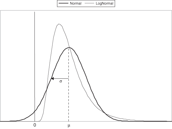
Figure 30.3: Comparison of normal versus log‐normal distribution functions with same mean, variance ( )
)
MODELING ASSET CHANGES
Normal distributions are commonly used to model the underlying asset value at option expiration. The focus is on the change in asset value from today until the expiration, with the change expressed either in percentage/proportional or absolute terms. Specifically, starting with asset value today, ![]() , a European‐style option depends on the unknown/random asset value at expiration,
, a European‐style option depends on the unknown/random asset value at expiration, ![]() .
.
Proportional Change
One way to model asset at expiration is to consider its changes over time via:
where ![]() is the continuously compounded random return over investment period
is the continuously compounded random return over investment period ![]() for the generic unknown future state of the world
for the generic unknown future state of the world ![]() :
:

This measure is also referred to as proportional return, percentage return, or log return. Its standard deviation is referred to as percentage, proportional or log volatility, or just volatility:

Assuming that the percentage return is Normal
implies that the asset value at expiration will be Log‐Normal:
This Log‐Normal distribution is somewhat close to the empirical distributions observed for equities—although the empirical/realized distributions tend to have fatter tails than Log‐Normal—and is commonly used for Equity/FX/Commodity options. The original Black‐Scholes‐Merton Formula for European call and its variant, Black's Call Formula for futures/forwards, were derived assuming this dynamic for the evolution of asset prices in a risk‐neutral world (![]() ). Specifically, Black's Call Formula is
). Specifically, Black's Call Formula is

where

Absolute Change
Another way to model change is to focus on the absolute change, ![]() , and to model this random change as a Normal r.v.
, and to model this random change as a Normal r.v.
Under this model, the underlying can take on negative values at expiration, and while inappropriate for equities/FX/commodities, it turns out to be the lesser of the two evils for interest rates, and has become the dominant base‐case model for interest rate derivatives. With this dynamic in a risk‐neutral setting (![]() ), we get the following formula
), we get the following formula

where

Note that ![]() is a measure of the money‐ness of the option as it expresses the distance between the forward versus the strike,
is a measure of the money‐ness of the option as it expresses the distance between the forward versus the strike, ![]() , expressed in units of standard deviation,
, expressed in units of standard deviation, ![]() . A similar interpretation can be given to
. A similar interpretation can be given to ![]() for Log‐Normal dynamics.
for Log‐Normal dynamics.
Put‐Call Parity
To derive the value of a European put, we would consider two portfolios:
- (1) A
 ‐expiry call option with strike
  , and cash holding equal to the Present Value of
  , that is,
  .
. - (2) A
 ‐expiry put option with strike
  , and the underlying asset,
  .
.
If the underlying asset has no interim cash‐flows until ![]() , then the two portfolios will have the same value,
, then the two portfolios will have the same value, ![]() , at expiration
, at expiration ![]() . Therefore, they must have the same value today (
. Therefore, they must have the same value today (![]() ), and we must have:
), and we must have:
This identity is called put–call parity, and holds for European‐style options on underlyings with no interim cash‐flows.
In particular, when the strike equals the At‐The‐Money‐Forward (ATMF) value of the asset, ![]() , then the call and put prices coincide:
, then the call and put prices coincide: ![]() .
.
GREEKS
Recall that Black's Formulae were obtained as special instances of Risk‐Neutral Valuation under Normal distributions for proportional or absolute returns. We should not forget that Risk‐Neutral Valuation gives the same value as a self‐financing replicating portfolio. The question arises as to what happened to the replicating portfolio, and how do we replicate an option's payoff? The answer lies in the Greeks.
Recall that in our binomial setting, the replicating portfolio was ![]() units of the underlying asset financed via a risk‐free loan. The
units of the underlying asset financed via a risk‐free loan. The ![]() amount had to be (dynamically) changed in response to market movements. In the simple 1‐step binomial model, we computed
amount had to be (dynamically) changed in response to market movements. In the simple 1‐step binomial model, we computed

which can be interpreted as the sensitivity of the option price with respect to the underlying asset.
In the limit, ![]() , and the replicating portfolio consists of
, and the replicating portfolio consists of ![]() units of a forward contract on the asset. This is called the Delta of the option. The Delta is a number between 0 and 1, and expresses how much of the forward asset is needed to replicate the option payoff. For Log‐Normal dynamics, it is measured as
units of a forward contract on the asset. This is called the Delta of the option. The Delta is a number between 0 and 1, and expresses how much of the forward asset is needed to replicate the option payoff. For Log‐Normal dynamics, it is measured as ![]() , while for Normal it is
, while for Normal it is ![]() .
.
As we saw in the 2‐step binomial model, the Delta changes. The rate of change of Delta with respect to the underlying is called Gamma and is defined as ![]() . Gamma measures the curvature of the option payoff, and is also called the convexity.
. Gamma measures the curvature of the option payoff, and is also called the convexity.
The intrinsic value of an option is its value at expiration, and the Time Value of an option is the difference between the option value and its intrinsic value. Time Value converges to 0 as one gets closer to expiration. Theta or time‐decay is defined as the rate of change of option value due to time ![]() . An option holder typically loses Time Value as one gets closer to expiry.
. An option holder typically loses Time Value as one gets closer to expiry.
Finally, the sensitivity of an option with respect to volatility ![]() is called Vega.
is called Vega.
Gamma versus Theta
As seen in Figure 30.4, Black call formula is a convex function of the underlying, and its delta changes when the underlying moves. The dynamic rebalancing of the replicating portfolio is primarily the result of this convexity, and it confers a systematic edge to the replicating portfolio. Loosely said, a delta‐hedged replicating portfolio consisting of a financed position of delta ![]() units of the underlying will need to get rebalanced as forwards move. For the option holder, be it a call or a put, it requires reducing/increasing the position as the underlying appreciates/depreciates, that is, the option holder will have to buy‐low, sell‐high to replicate the option payoff! The amount of this excess P&L of a delta‐hedged option is
predominantly
units of the underlying will need to get rebalanced as forwards move. For the option holder, be it a call or a put, it requires reducing/increasing the position as the underlying appreciates/depreciates, that is, the option holder will have to buy‐low, sell‐high to replicate the option payoff! The amount of this excess P&L of a delta‐hedged option is
predominantly ![]() , similar to the convexity P&L of a duration‐neutral portfolio of bonds.
, similar to the convexity P&L of a duration‐neutral portfolio of bonds.
A delta‐hedged long option position experiences two dominant P&Ls: it loses Time Value every day, and it gains a gamma P&L as the position is rebalanced (delta's changed). Note that the gamma P&L is incurred whether the asset moves up or down. This is shown in Figure 30.4 for a call option. The typical (expected) movement of the forward asset over a short interval time ![]() is prescribed by volatility as
is prescribed by volatility as ![]() . Each move in the forwards incurs a gamma P&L, and passage of time leads theta P&L due to loss of Time Value. Black's formula is the correct computation of the expected value of the sum of these two P&Ls over the life of the option.
. Each move in the forwards incurs a gamma P&L, and passage of time leads theta P&L due to loss of Time Value. Black's formula is the correct computation of the expected value of the sum of these two P&Ls over the life of the option.

Figure 30.4: Gamma P&L versus time decay for a European call option
Digitals
A digital call option ![]() has unit payoff if the asset
has unit payoff if the asset ![]() at expiration
at expiration ![]() is above the strike
is above the strike ![]() :
:

Similarly, a Digital put has a unit payoff if the asset at expiration is below the strike ![]() :
:
Cheat Sheet
Tables 30.1 and 30.2 summarize various Black formulae and their Greeks. All of these are for European options without the discounting from payment date to today. Recall that
Table 30.1: Black Log‐Normal Formulae
| Premium | Delta | |
| Call | ||
| Put | ||
| Digi‐Call |  |
|
| Digi‐Put |  |
Table 30.2: Black Normal Formulae
| Premium | Delta | |
| Call | ||
| Put | ||
| Digi‐Call |  |
|
| Digi‐Put |  |
 |
CALL IS ALL YOU NEED
One can continue along the above lines to derive analytical formulae for European‐Style options with more complicated payoffs. In practice, however, the call and digi‐call formulae are all one really needs to evaluate European‐style options. Indeed, any real‐world option payoff is economically equal to—or can be approximated arbitrarily closely—via a portfolio of calls and/or digi‐calls. Hence calls and digi‐calls serve as the salient building blocks of European‐Style options.
The following is a list of some common European‐style (single‐exercise) payoffs encountered in practice:
- Straddle—A put and call with same strike
 .
. - Strangle—A
 ‐put and
  ‐call where
  .
. - Collar—Being long a collar is being long a
 ‐call, and short a
  ‐put with
  . The strikes
  are usually chosen around the forward rates, so that the package is worth 0, that is, a costless‐collar.
 - Risk‐Reversal—Long a call at
 and short a put at
  is called a
  ‐total‐width (or
  on each side) risk‐reversal. Under Normal dynamics with no skews, a risk‐reversal should be worth zero. Traders track the price of various‐width risk‐reversals to discover the implied skews in the market.
 - Call/Put Spread—Being long a call‐spread is being long a
 ‐call, and short a
  ‐call, with
  .
. - Ratio–Most common is a
 (1 by 2) ratio. Being long a
  call ratio means being long one
  ‐call, and short two
  ‐calls. Some traders track the implied market skews by setting
  ,
,  , and solving for
  that would make the ratio costless, the higher the call‐skew, the higher the solved
  .
. - Fly—Being long a call‐fly is being long one
 ‐call, short two
  ‐calls, and long one
  ‐calls, with
  , and
, and  . This is usually used to pin down and express strong views on the setting of Libor at expiration, leading to Pin Risk for the option‐seller.
 - Digitals—Digi‐calls, Digi‐puts. Due to their high gamma, these are usually sold as a conservative (from seller's point of view) call or put spreads, with the strikes chosen to be 10–20 basis points apart (called the “width of the ramp”).
- Knock‐in Call/Put—A
 ‐strike call with
  ‐knock‐in (
 ) has the same payoff of a
  ‐call, but only if the underlying is above
  at expiration. The payoff is zero if the underlying is below
  at expiration. This can easily be priced as a
  ‐call plus a
  ‐Digi‐Call with payoff
  .
.
These are shown in Figure 30.5. All of the above products can be priced via Black's Normal/Log‐Normal formulae, as the payoffs are simple portfolios of different‐strike calls/puts and digi‐calls/puts.

Figure 30.5: Common European‐style payoffs
INTEREST RATE OPTIONS
The Black‐Scholes‐Merton Formula, and its Black variant for futures was historically derived for non‐interest‐rate related underlying assets (Equities, FX, Commodities), and under the assumption that interest rates are non‐random. When interest rate options (cap/floors, swaptions) were introduced, traders co‐opted these formulas and applied them to interest rates. While everyone recognized that the formulae need to be adjusted since interest rates are not traded assets, and are random, nevertheless, in the absence of any other simple alternatives, Black's Formula became and still continues to be the standard option pricing formula for flow products.
For most market practitioners, Black's formula is mostly a quoting mechanism, and also a guide on calculating deltas needed to replicate the option payoff under the assumed (often too simplistic) dynamics. Just like bonds, ultimately all interest‐rate options trade on price. And just like bonds where implied flat yields are calculated, implied vols are calculated to help assess the fairness of the quoted option prices.
For interest rate options, since ATMF straddles have little duration risk, and are predominantly a function of the volatility, ATMF straddles are actively quoted and traded. Option traders are in the business of taking and managing volatility risk, not duration or spread risk, as each option desk will try to maintain a delta‐neutral position and takes only volatility risk. By monitoring and trading ATMF straddles, they are then trading volatility itself.
Initially, Black's Log‐Normal formulae were co‐opted for interest rate products. In recent years, however, most traders have switched to the Normal dynamics as the base case, and brokers quite often quote Normal vols alongside prices in preference to Log‐Normal vols.
MARKET PLAYERS
As with any other derivative, interest rate options can be used for hedging or for speculation.
Hedging, Protection
Mortgage servicing companies often buy swaptions to hedge the negative convexity of their servicing portfolios. Insurance companies typically buy cap/floors to hedge their guaranteed‐payoff annuity products.
Speculation, Penny Options, Lottery Tickets
Hedge funds typically utilize interest rate options to express a view on the terminal setting of interest rates at expiration. Rather than entering into a forward agreement, they usually buy cheap out‐of‐the‐money options to cap the downside to the premium paid, while benefitting handsomely if their view is borne out. These buyers do not hedge the interest rate options, except sometimes under a favorable outcome before expiration to lock in profit, or by rolling the strike.
Gamma Trading, Realized versus Implied Vol
The dominant P&L of short‐dated (6m and under) options when delta‐hedged is due to their gamma. If the actual realized volatility turns out to be higher than the implied volatility paid through the up‐front premium, then delta‐hedging can be a source of profit for a long position in an option. Similarly, a seller of an option profits when realized volatility is smaller than implied vol.
Vega Trading, Supply/Demand
For longer‐dated options (1y and longer expiries), the dominant P&L is due to changes in implied volatility, that is, their vega. These changes in implied vols are primarily due to supply and demand of volatility. For example, a large hedging program by a servicing company can drive up volatilities in one sector, while the hedging needs of exotics desks can pressure a specific sector of the volatility surface. An astute anticipation of these flows allows one to take a position—usually via straddles in order to minimize delta‐hedging needs—in vega pieces, and then unwinding the position for profit/loss after a favorable/unfavorable outcome. As these trades can span a few months for the flows to be realized, one needs to consider the volatility carry (loss of time‐value) and roll‐down (slope of the volatility surface along expiry).
CAPLETS/FLOORLETS: OPTIONS ON FORWARD RATES
A caplet/floorlet is a European option on a rate, typically the benchmark interest rate, say 3m Libor. A typical caplet/floorlet on 3m Libor is based on a single calculation period: ![]() . At expiration
. At expiration ![]() the market rate is compared to the strike
the market rate is compared to the strike ![]() , and the option payoff is accrued for the duration of the calculation period, and paid at the end of the calculation period
, and the option payoff is accrued for the duration of the calculation period, and paid at the end of the calculation period ![]() . For example, a 6m‐expiry 2% caplet on 3m Libor has the following payoff 9m from today:
. For example, a 6m‐expiry 2% caplet on 3m Libor has the following payoff 9m from today:
per unit notional, where ![]() is the accrual fraction.
is the accrual fraction.
Market practice is to use Black's formula to price options on futures. For a given calculation period ![]() , the risk‐neutral formula for a caplet on a rate
, the risk‐neutral formula for a caplet on a rate ![]() is calculated as:
is calculated as:
and it is further assumed that a forward rate is a tradeable asset, hence Black's call formula is used to evaluate the ![]() term. Similarly, for floorlets, the payoff
term. Similarly, for floorlets, the payoff  is evaluated using Black's put formula.
Caps/Floors
A cap/floor is simply a portfolio of caplets/floorlets, all having the same strike. For example, a 2y 2% quarterly cap on 3m Libor is a collection of 8 caplets based on 8 calculation periods: ![]() , where each caplet's strike is 2%. Each caplet/floorlet is valued using Black's formula using its own (depending on its expiration date) volatility, and the value of the cap/floor is simply the sum of all these values.
, where each caplet's strike is 2%. Each caplet/floorlet is valued using Black's formula using its own (depending on its expiration date) volatility, and the value of the cap/floor is simply the sum of all these values.
An ![]() (pronounced
(pronounced ![]() by
by ![]() ) forward cap/floor is a cap/floor starting
) forward cap/floor is a cap/floor starting ![]() years from today, and maturing
years from today, and maturing ![]() years from today. So a
years from today. So a ![]() cap is a 1y cap, starting in 1y; a
cap is a 1y cap, starting in 1y; a ![]() cap is a 2y cap, starting in 3y.
cap is a 2y cap, starting in 3y.
In practice, only prices of a few caps/floors are actively quoted in the form of cap‐floor straddles. Typical maturities are 1y, ![]() ,
, ![]() ,
, ![]() ,
, ![]() ,
, ![]() for USD cap/floors. For example, a
for USD cap/floors. For example, a ![]() USD “cap‐floor straddle” quoted as 25 cents denotes a price of $250,000 for a package consisting of one $100mm
USD “cap‐floor straddle” quoted as 25 cents denotes a price of $250,000 for a package consisting of one $100mm ![]() quarterly cap (4 caplets) and one $100mm
quarterly cap (4 caplets) and one $100mm ![]() quarterly floor (4 floorlets). The common strike for all caplets/floorlets is chosen so that all caplet
quarterly floor (4 floorlets). The common strike for all caplets/floorlets is chosen so that all caplet![]() floorlets pairs (one pair for each expiration) are close to ATMF.
floorlets pairs (one pair for each expiration) are close to ATMF.
A final note is that for spot‐start caps/floors, the first caplet/floorlet is ignored, so a 1y quarterly cap is really a 3m ![]() 1y cap, and has actually 3 caplets:
1y cap, and has actually 3 caplets:  . A forward quarterly 1y cap, say
 ![]() , however has 4 caplets.
, however has 4 caplets.
Options on Euro‐Dollar Futures
Options on Euro‐dollar futures trade at Chicago Mercantile Exchange (CME) and are quoted in Euro‐dollar ticks ($25 per contract). Options on Euro‐dollar futures are treated as caplets/floorlets, using Black's formula to evaluate them.
Caplet Curve  ED Options
  Cap/Floors
Options on the first few ED contracts are fairly liquid, and can be used to back out the implied volatilities of 3m‐Libor rates for the relevant expirations. Since a dealer cap/floor book consists of many expiration dates, with each expiry having its own volatility, a caplet curve is needed to mark this book. The caplet curve is a graph of implied‐vols of options on the benchmark floating index versus expiration.
For USD, the instruments used to construct this curve are ATMF options (or strikes as close to forwards as possible) on ED1, ED2,…, and a series of cap/floor straddles: ![]() ,
, ![]() ,
, ![]() ,
, ![]() ,
, ![]() . Since each cap/floor straddle consists of multi‐expiration caplet+floorlet pairs, with each expiration requiring its own volatility, a bootstrap+interpolation routine is typically used to back out the implied vol for each expiration. A common procedure is to use implied vols from ED futures options for the first few expiries, and use a parametric shape for the rest of the curve.
. Since each cap/floor straddle consists of multi‐expiration caplet+floorlet pairs, with each expiration requiring its own volatility, a bootstrap+interpolation routine is typically used to back out the implied vol for each expiration. A common procedure is to use implied vols from ED futures options for the first few expiries, and use a parametric shape for the rest of the curve.
EUROPEAN‐STYLE SWAPTIONS
An ![]() ‐year into
‐year into ![]() ‐year receiver/payer swaption with strike
‐year receiver/payer swaption with strike ![]() is an
is an ![]() ‐year European option to receive/pay the fixed rate
‐year European option to receive/pay the fixed rate ![]() in an
in an ![]() ‐year swap. Let us focus on a Right‐to‐Pay (RTP) or payer swaption. At option expiry, if (and only if) the
‐year swap. Let us focus on a Right‐to‐Pay (RTP) or payer swaption. At option expiry, if (and only if) the ![]() ‐year par swap rate
‐year par swap rate ![]() is above the strike
is above the strike ![]() , then it is advantageous to exercise the option and pay
, then it is advantageous to exercise the option and pay ![]() (below market). Otherwise, if
(below market). Otherwise, if ![]() , the option holder will not exercise the option, as it is cheaper to pay
, the option holder will not exercise the option, as it is cheaper to pay ![]() in a market swap rather than the higher rate
in a market swap rather than the higher rate ![]() .
.
If ![]() , the option will get exercised and the option owner will pay
, the option will get exercised and the option owner will pay ![]() for the next
for the next ![]() years. He could also (conceptually) receive fixed in a par swap (worth 0), that is, receiving
years. He could also (conceptually) receive fixed in a par swap (worth 0), that is, receiving ![]() and pay floating for
and pay floating for ![]() ‐years. Netting these two swaps, the floating legs cancel out, and effectively one is paying
‐years. Netting these two swaps, the floating legs cancel out, and effectively one is paying ![]() and receiving
and receiving ![]() for the next
for the next ![]() ‐years on the payment dates of the underlying swap. Assuming that the underlying swap is semi‐annual, let
‐years on the payment dates of the underlying swap. Assuming that the underlying swap is semi‐annual, let ![]() be the payment dates for the fixed leg of the swap. The economic value of the payer swaption at expiration
be the payment dates for the fixed leg of the swap. The economic value of the payer swaption at expiration ![]() then is
then is

where ![]() is the random discount‐factor curve at
is the random discount‐factor curve at ![]() .
.
According to risk‐neutral valuation, today's price of this option is simply the expected discounted value of the above payoff. This is approximated as follows:
where ![]() is today's value of an annuity that pays unit payoff on the underlying forward swap's payment dates, and the last term is evaluated using Black's call formula.
is today's value of an annuity that pays unit payoff on the underlying forward swap's payment dates, and the last term is evaluated using Black's call formula.
Similarly, the formula for a receiver swaption is
where the last term is evaluated using Black's put formula using forward swap rates.
Swaptions in Practice
Inter‐dealer‐brokers maintain ATMF straddle prices for various expirations and maturities, and communicate bids/offer prices for specific straddles between dealers. They also maintain a general swaption price grid for all expiries and maturities in electronic format (broker screens), update them periodically during the day, and send a final settlement grid at end of day. Alongside the price, they might also quote the implied Log‐Normal or Normal vol, but that is mostly for informational purposes, as at the end of the day, price is king (see Tables 30.3 and 30.4). So a 1m‐into‐2y swaption straddle is trading at 29 cents ($290,000 per $100 million notional), and this price is equivalent to Black Normal vol of 68.3bp/annum.
Table 30.3: A Swaption Straddle Price Grid (Cents)
| Underlying Swap Term | ||||||||||
| 1y | 2y | 3y | 4y | 5y | 7y | 10y | 15y | 30y | ||
| “Gamma” Expiries | 1m | 9 | 29 | 43 | 60 | 78 | 103 | 134 | 175 | 242 |
| 3m | 22 | 57 | 87 | 115 | 144 | 188 | 245 | 324 | 446 | |
| 6m | 34 | 80 | 123 | 162 | 199 | 262 | 339 | 443 | 608 | |
| “Vega” Expiries | 1y | 60 | 119 | 174 | 227 | 276 | 363 | 469 | 608 | 837 |
| 2y | 86 | 169 | 246 | 318 | 385 | 502 | 645 | 833 | 1,124 | |
| 3y | 103 | 201 | 291 | 376 | 454 | 594 | 760 | 975 | 1,316 | |
| 5y | 120 | 232 | 337 | 434 | 524 | 680 | 876 | 1,118 | 1,500 | |
| 7y | 124 | 238 | 347 | 448 | 542 | 704 | 897 | 1,136 | 1,497 | |
| 10y | 120 | 230 | 333 | 428 | 516 | 669 | 855 | 1,075 | 1,401 | |
Table 30.4: Implied Black Normal Vols (bp)
| 1y | 2y | 3y | 4y | 5y | 7y | 10y | 15y | 30y | |
| 1m | 43.2 | 68.3 | 70.4 | 75.5 | 80.5 | 79.9 | 78.7 | 77.8 | 75.8 |
| 3m | 57.0 | 77.6 | 80.4 | 81.9 | 83.8 | 82.5 | 81.4 | 81.1 | 79.0 |
| 6m | 65.0 | 77.4 | 81.6 | 82.6 | 83.5 | 82.8 | 81.1 | 79.8 | 77.4 |
| 1y | 81.9 | 83.6 | 83.9 | 84.4 | 84.3 | 83.5 | 81.6 | 79.9 | 77.7 |
| 2y | 88.5 | 89.2 | 88.6 | 88.4 | 88.0 | 86.4 | 84.1 | 82.1 | 78.3 |
| 3y | 91.6 | 91.4 | 90.7 | 90.2 | 89.7 | 88.4 | 85.8 | 83.3 | 79.3 |
| 5y | 92.2 | 91.4 | 91.3 | 90.6 | 89.9 | 88.0 | 86.1 | 83.2 | 78.6 |
| 7y | 90.7 | 89.4 | 89.2 | 88.8 | 88.4 | 86.8 | 84.0 | 80.5 | 74.6 |
| 10y | 87.1 | 86.0 | 85.5 | 84.9 | 84.4 | 82.6 | 80.2 | 76.2 | 69.7 |
When trading ATMF straddles, a price is agreed on, and the next step is to agree on the forward swap rate. Due to their curve differences, each side might see the ATMF rate at slightly different values. However, since straddles will have little PV01, both sides agree on a rate (perhaps aided by the broker).
If instead of straddles, a receiver or payer swaption is traded, one needs to specify whether the hedge/delta is exchanged or not. The standard hedge, regardless of the option strike, consists of a delta‐weighted amount of a forward swap (struck at the forward swap rate, so with 0 value).
If the trade is with the delta/hedge, then one first sets the option price, and the forward rate and the size of the hedge are agreed upon later. In this case, similar to trading straddles, since the PV01 of the combined position (option+hedge) are small, minor rate or delta differences as seen by different sides are (usually) amicably settled.
If the trade is done without the delta/hedge, then a sufficient extra (hedging) premium is built into the option price to cover the subsequent hedging bid/offer cost. The natural preference of an option trader is to transact options with delta, thereby just trading volatility.
For swaption expiries and maturities that do not fall on the grid, one typically uses linear interpolation in square root of time‐to‐expiry on the expiry axis, and linear interpolation on the maturity axis.
Swaption Settlement
At expiration, swaptions can be either physical or cash‐settled. For physical settlement, the owner of an in‐the‐money receiver/payer swaption will enter into a plain‐vanilla swap where he will receive/pay the strike as the fixed rate. Physical settlement is the preferred method for swaptions that are sufficiently (say more than 10bp) in the money, even if the originally agreed‐upon settlement method is cash.
Cash‐settlement involves determining the market par swap rate at expiration time, and then agreeing upon the value of a swap with fixed rate equal to the strike instead of the par‐swap rate. As we saw before, the economic value of an in‐the‐money swaption struck at ![]() when par‐swap rate is
when par‐swap rate is ![]() is an annuity of
is an annuity of ![]() bp's for RTP (
bp's for RTP (![]() for RTR) for the length of the swap. Therefore, both parties must agree upon the size (
for RTR) for the length of the swap. Therefore, both parties must agree upon the size (![]() ) and the Present‐Value of this annuity.
) and the Present‐Value of this annuity.
Since the strike ![]() is by contract, the swaption counterparties first have to agree on the par‐swap rate
is by contract, the swaption counterparties first have to agree on the par‐swap rate ![]() at expiration time. This can be mutual agreement, or polling dealers, or some other method as specified in the option confirm. For generic USD swaptions, the standard is to use the 11:00am fixing of swap rates. Once the size of the annuity (
at expiration time. This can be mutual agreement, or polling dealers, or some other method as specified in the option confirm. For generic USD swaptions, the standard is to use the 11:00am fixing of swap rates. Once the size of the annuity (![]() ) is known, the counterparties have to then agree on its PV.
) is known, the counterparties have to then agree on its PV.
There are two methods to calculate the PV of the annuity. The first method (the
standard for USD swaptions) is to use a discount factor curve to PV the annuity. For example for an ![]() ‐year swap with
‐year swap with ![]() coupons per year, with payment dates
coupons per year, with payment dates ![]() , each party needs to compute:
, each party needs to compute:

As each counterparty can have a different discount‐curve (even using the same rate ![]() as the
as the ![]() ‐year par‐swap rate), a bit of horse‐trading precedes an amicable cash‐settlement of the swaption. This method does not have a standard name, and can be referred to as “cash‐settlement off the curve” or cash‐settlement “USD‐style.”
‐year par‐swap rate), a bit of horse‐trading precedes an amicable cash‐settlement of the swaption. This method does not have a standard name, and can be referred to as “cash‐settlement off the curve” or cash‐settlement “USD‐style.”
The second cash‐settlement method is to PV the annuity using the annuity formula from bonds, using the agreed‐upon swap rate as the yield. This method is the standard for European currencies, and is referred to as “cash‐settlement via annuity (or IRR) method.” For an ![]() ‐year swap with
‐year swap with ![]() coupons per year, the payoff is
coupons per year, the payoff is

SKEWS, SMILES
In a perfect Black world, asset prices evolve (Normally, Log‐Normally) with a single volatility parameter. The price of options then can be obtained once we know this volatility, or alternatively, given a price, we can back out the implied volatility. In practice, it is observed that option prices with the same expiration date but different strikes give rise to different implied Black volatilities. Typically, for options with strikes lower than ATMF, the implied volatility goes up, and this effect is called skew. Also out‐of‐the‐money options in either direction (high or low strikes) generally have higher implied Black volatilities than ATMF options. This effect is called volatility smile.
The existence of skews and smiles means that the implied distribution of the assets is more complicated than what is posited by Black (Normal, Log‐Normal) model, and has given rise to a cottage industry of searching for the right model for skew and smile. Amongst the models proposed are mixture models, Constant Elasticity of Variance (CEV) models, Stochastic volatility models (SABR amongst them), Jump‐Diffusion models, and Fractional Brownian Motion models. While each of these models have its merits, they collectively suffer from the fact that they are modeling the wrong thing!
Skews and smiles are predominantly driven by supply and demand. If a majority of clients are worried about higher rates, and are buying high‐strike payers to protect themselves, payer swaptions go up in price (and hence in implied vol). Alternatively, if the fear is for low rates, then low‐strike receivers go up in premium/vol. On a day‐to‐day basis, vol traders perceive the skew/smile as a measure of liquidity rather than the implied distribution of rates. Supply/demand patterns change quickly in response to market sentiments/news, and it is implausible to ascribe these changes to market's view on a meaningful distribution of rates for the life of the option.
Maintaining/Populating Volatility Surface, Cubes
For swaptions, it is customary to maintain a Black volatility cube, that is, a volatility for each expiration, swap maturity, and strike. Some desks maintain vols for a series of absolute (1%, 1.25%, 1.5%,…, 9.75%, 10%,…) strikes, while most desks maintain vols for a series of relative (ATMF, ATMF![]() 25bp, ATMF
25bp, ATMF![]() 50bp, ATMF
50bp, ATMF![]() 100bp,…) strikes. A similar procedure is used for caplet vol curves.
100bp,…) strikes. A similar procedure is used for caplet vol curves.
As one might imagine, the task of maintaining ATMF volatility surfaces (Expiration, Swap Maturity) and cubes (Expiration, Maturity, Strike) is arduous. Depending on the market, there are 10–20 expirations, 10–20 maturities, and 10–20 strike levels (absolute or relative), hence a rates option trader needs to maintain on the order of 1000 live prices! Given that on a typical trading day, only a few (10–20) swaptions and cap/floors trade, most desks keep active watch on certain anchor vols, and derive other neighboring vols via linear/ratio interpolation/extrapolation. For example, in USD, 1m2y, 1m5y, 1m10y, 3m10y, 1y1y, and 5y5y can serve as the anchor vols. Once we know these vols, the vol of 1m3y, 1m4y or 2m10y can plausibly (in the absence of actual markets) be backed out via interpolation.
The market for skews is less active than ATMF options. Most desks select a skew model (SABR, CEV,…) and calibrate the few model parameters to any observed skew markets, quoted commonly through risk‐reversals: The difference between the price of an out‐of‐the‐money payer swaption versus an equally out‐of‐the‐money receiver. For Normal dynamics, in the absence of any skew these prices should be the same, as the Normal distribution is symmetric. Hence, when a difference exists, it is indicative of Non‐Normality or skew. Using these skews markets, volatility traders then populate the cube using these few parameters. Hence the role of skew models is primarily to reduce the dimension of the problem from 1000's to 100's (potentially each Expiration/Swap‐Term pair can have its own set of parameters).
CMS PRODUCTS
A CMS (Constant Maturity Swap) rate is simply the par‐swap rate for a given tenor, and a CMS Swap is the periodic exchange of a CMS rate versus either a fixed rate, or more typically versus Libor. For example, a USD 2‐year CMS‐10y versus Libor consists of a standard quarterly, Act/360 floating leg based on 3m Libor, versus the quarterly fixing and payment (accrued 30/360) of 10‐year par swap rate on the CMS leg, with both legs spanning 2 years. Since the tenor of the underlying CMS rate does not coincide with the length of the calculation period, the replication argument for plain vanilla Libor legs does not hold, and one cannot simply discount the forward par‐swap rates. Still, there is a strong temptation to do this, and one typically values CMS resets by first calculating the forward swap rate, and then adjusting them by a CMS Convexity Adjustment. The term convexity adjustment arises in different contexts in interest rate derivatives, and is usually a red flag that a certain level of fudging is going on. Specifically, convexity adjustments are a quick‐and‐dirty way of getting the right answer by applying the wrong method, for example discounting the forward rates for CMS products. This obviously pre‐supposes that we have the right answer, or at least an idea of what the right answer should be!
For CMS‐based payoffs, it is first recognized that while the payoff is linear in the underlying CMS rate, a replicating portfolio would consist of forward swap positions. Recalling that receiving in a swap is economically equivalent to paying par for a forward bond, the graph of the forward swap value is a convex function of the underlying swap rate, analogous to the price/yield graph for bonds. For a CMS‐based swap, we therefore are hedging a linear payoff (CMS rate) with a non‐linear/convex payoff (Forward Swap). The hedge for receiving the CMS‐rate is to pay in a PV01‐equivalent amount of a forward swap. This hedge, however, confers a systematic advantage to the CMS‐receiver, the size of which depends on the curvature/convexity of the forward swap versus the swap rate, and the expected size of the deviation of the realized swap rate at reset‐date versus its forward value. As no free lunch goes untaxed in markets, the CMS‐payer will charge the receiver for this free lunch by adjusting the forward swap rate upwards by the convexity adjustment. Note that this adjustment is only used to calculate the PV of future payments, the actual payment on payment date is simply the CMS rate observed at the fixing date (with no adjustment).
The fair level of this CMS convexity adjustment will require a model of the distribution of future swap rates at each reset date in a risk‐neutral setting. In lieu of this, the following heuristic argument is invoked to obtain a quick and dirty formula. Using bonds as proxies for swaps, we start with the following approximaton:
where ![]() is the forward par‐swap rate, and
is the forward par‐swap rate, and ![]() is the standard Bond Price‐Yield Formula. It is recalled that forward prices must equal expected prices in a risk‐neutral world, hence
is the standard Bond Price‐Yield Formula. It is recalled that forward prices must equal expected prices in a risk‐neutral world, hence ![]() , and
, and
Finally, we approximate
to arrive at the following CMS Convexity Adjustment Formula:

where ![]() are the number and frequency of coupon payments for the underlying forward (
are the number and frequency of coupon payments for the underlying forward (![]() ) bond/swap, and
) bond/swap, and ![]() is the time to its reset. While very heuristic and approximate, the above formula due to its simple structure is widely used and in preference to more elaborate models.
is the time to its reset. While very heuristic and approximate, the above formula due to its simple structure is widely used and in preference to more elaborate models.
CMS Curve Options
In the past couple of years, options on the slope of swap curve have become popular. These are referred to as CMS Curve Options, as they are simple cap/floors on the difference between two CMS rates. For example, a CMS 2y–10y curve caplet with strike ![]() is based on the following payoff
is based on the following payoff
The simplest method of evaluating CMS curve products is to use Black's Normal model—Log‐Normal would be inappropriate since spreads can go negative, and zero or negative strikes are not uncommon—for the spread: ![]() , and extract the Normal vol of the spread from the swaption Normal volatilities via:
, and extract the Normal vol of the spread from the swaption Normal volatilities via:
where ![]() are the swaption normal vols for the CMS rates, and
are the swaption normal vols for the CMS rates, and ![]() is the correlation between them.
is the correlation between them.
Contingent Curve Trades
While CMS curve options are the most direct way of taking a view on the slope of the swap curve, one may put on a conditional curve trade using European swaptions, since curve trades are usually directional: The front end of the swap curve is more volatile than the long end as it is more sensitive to central bank policies, and the front end typically leads the long end in either increasing or decreasing rate environments. Therefore, in a tightening (rising rate) environment, the short‐term swap rates move more than longer‐term swap rates, leading to flattening of the swap curve. This is referred to as bear‐flattening–“bear” since bond prices are dropping in rising rate environments. Similarly, in an easing (falling rate) environment, short‐term rates fall more than long‐term rates, leading to bull‐steepening. As such, one would want to be in a flattener in bearish environments, while steepeners are preferred in bullish environments.
To be long a steepener, one can either be long the curve via swaps (long the front end, short the back‐end), using either spot or forward swaps. Instead, one can be in a conditional steepener by buying a swaption receiver into the shorter maturity, while selling a swaption receiver into the longer maturity. The size of each swaption is chosen so that if they are both in the money at expiration, each swap will have the same PV01, while the strikes of the swaptions are chosen so that the package is zero‐cost: Zero‐cost bull‐steepener (sometimes called conditional or contingent call‐call). Similarly, a zero‐cost bear‐flattener consists of a pair of payer swaptions with strikes chosen to make the package zero‐cost.
BOND OPTIONS
While not strictly a “Rates” product, bond options are sometimes quoted by flow options desks. The typical expiration for these options is relatively short (a few days or weeks), and are usually priced and hedged using Black's Log‐Normal formula, driven by price volatility. As the market for bond options is relatively thin, this price volatility is backed out from yield volatility using the following heuristic argument: Yield log‐volatility ![]() measures a one standard deviation percentage change in yields:
measures a one standard deviation percentage change in yields:

while price log‐volatility ![]() measures a one standard deviation percentage change in prices:
measures a one standard deviation percentage change in prices:
One can relate change in prices due to change in yields:

therefore

A common approach is to derive the yield volatility from a similar‐maturity swaption volatility using simple regression analysis. For example, when asked to quote a 1m option on the current U.S. Treasury 10y bond (CT10), one can perform a regression analysis on the relationship between 10y Treasury yields versus 10y swap rates, and multiply the 1m‐into‐10y swaption volatility by the slope coefficient to arrive at a plausible yield volatility for CT10. By converting this yield vol into price vol, one can then price bond options using Black's Log‐Normal formula using clean forward and strike prices. Note that as option prices are based on replication using the underlying, the specific bond's financing (repo) rate rather than a generic risk‐free rate should be used in Black's formula.
Conditional Swap‐Spread Trades
While a swap spread trade involves a cash bond versus a swap, one can also enter into a conditional swap spread trade using swaptions and bond options. It is observed that swap spreads are typically directional. In falling rate environments, spreads generally “come in” (decrease), while they “go out” in increasing rate environments. To take advantage of this directionality, one would then like to be in a swap‐spread widening trade (long cash, pay in swaps) when interest rates are increasing, that is, a bearish‐widener. For a given cash bond, this can be achieved by selling a put option on the bond, while buying a PV01‐equivalent amount of a payer swaption with maturity identical to a bond: If both options finish in‐the‐money, the bond is put to us while we are paying in a matched‐maturity swap, that is, we are long the matched‐maturity swap spread of the bond when rates are increasing. The strikes of the put and swaption are usually chosen so that the package is cost‐less, typically by selecting one strike higher (in yield) than ATMF, and then solving for the other strike.
To take advantage of directionality in decreasing rate environments, one implements a bullish‐tightener by selling a call option on the bond and buying a PV01‐equivalent (if both options finish in‐the‐money) receiver swaption for a matched‐maturity swap, with strikes chosen so that the package is cost‐less, resulting in a zero‐cost call/reciever or bullish‐tightener.
A final note that due to relative low liquidity of bond options, most contingent swap‐spread trades are implemented using options on treasury futures contracts traded on Chicago Board of Trade (CBOT), with the future contract equated to Cheapest‐To‐Deliver (CTD) issue divided by its conversion factor.