CHAPTER 5
Enhancing Your Output with ODS
5.1 Concepts of the Output Delivery System
5.6 Customizing Titles and Footnotes
5.7 Customizing PROC PRINT with the STYLE= Option
5.8 Customizing PROC REPORT with the STYLE= Option
5.9 Customizing PROC TABULATE with the STYLE= Option
5.10 Adding Trafficlighting to Your Output
5.11 Selected Style Attributes
5.12 Tracing and Selecting Procedure Output
5.13 Creating SAS Data Sets from Procedure Output
5.1 Concepts of the Output Delivery System

You might think that procedures produce output. They don’t. Technically, procedures produce only data. Then they send the data to the Output Delivery System (ODS) which determines where the output should go and what it should look like when it gets there. That means the question to ask yourself is not whether you want to use ODS—you always use ODS. The question is whether to accept default output or choose something else.
ODS is like a busy airport. Passengers arrive by car and bus. Once at the airport, passengers check baggage, pass security, eventually board a plane, and fly out to their destinations. In ODS, data are like passengers arriving from various procedures. ODS processes each set of data and sends it off to its proper destination. In fact, different types of ODS output are called destinations. What your data look like when they get to their destination is determined by templates. A template is a set of instructions telling ODS how to format your data. These two concepts—destinations and templates—are fundamental to understanding what you can do with ODS.
Destinations SAS can send output to many different destinations. If you are satisfied with the default output, then you can skip the rest of this chapter. However, if you want more customized output, the features described in this chapter can help you. Here are the major ODS destinations:
|
CSV |
Comma-separated values |
|
EXCEL |
Microsoft Excel |
|
HTML |
Hypertext Markup Language |
|
LISTING |
plain text output |
|
OUTPUT |
SAS data set |
|
|
Portable Document Format |
|
POWERPOINT |
Microsoft PowerPoint |
|
PS |
PostScript |
|
RTF |
Rich Text Format |
|
WORD |
Microsoft Word document (pre-production in SAS 9.4 M6) |
HTML is the default destination for SAS Studio. HTML is also the default destination for SAS Enterprise Guide starting with release 8.1 (earlier versions use the proprietary format SASREPORT). Likewise, HTML is the default destination for the SAS windowing environment in Microsoft Windows and UNIX starting with SAS 9.3 (earlier versions use the LISTING destination). If you run SAS programs in batch or in other operating environments, the default destination is LISTING.
Most of these destinations are designed to create output for viewing on a screen or for printing. The CSV (Section 10.3), EXCEL (Section 10.5), and OUTPUT (Section 5.13) destinations, on the other hand, create data files or data sets.
Style and table templates Templates tell ODS how to format and present your data. The two most common types of templates are table templates and style templates (also called table definitions and style definitions). A table template specifies the basic structure of your output (which variable will be in the first column?), while a style template specifies how the output will look (will the headers be blue or red?). ODS combines the data produced by a procedure with a table template and together they are called an output object. The output object is then combined with a style template and sent to a destination to create your final output.

In ODS Graphics, instead of a table template, your data are combined with a graph template, and the final result is graphical output instead of tabular output. See Chapter 8 for more information about ODS Graphics.
You can create your own style templates using the TEMPLATE procedure. However, PROC TEMPLATE’s syntax is rather arcane. Fortunately, there are other ways to control and modify output. The quickest and easiest way to change the look of your output is to use one of the many built-in style templates. To view a list of the style templates available on your system, submit the following PROC TEMPLATE statements:
PROC TEMPLATE;
LIST STYLES;
RUN;
Here are a few of the built-in style templates:
|
ANALYSIS |
HTMLBLUE |
MINIMAL |
RTF |
STATISTICAL |
|
BARRETTSBLUE |
JOURNAL |
PEARL |
SASWEB |
|
Notice that RTF is the name of both a destination and a style. Some styles work better with certain destinations than with others. HTMLBLUE is the default style for HTML output, RTF is the default style for RTF output, and PEARL is the default style for output sent to the PDF and PS destinations.
While all procedures that produce printable output allow you to use style templates to control the overall look of that output, the PRINT, REPORT, and TABULATE procedures allow you to do something special. With these three procedures, you can use the STYLE= option directly in the PROC step to control individual features of your output without having to create a whole new style template. Sections 5.7 to 5.11 discuss how to do this.
5.2 Creating HTML Output
When you send output to the HTML destination, you get files in Hypertext Markup Language format. These files are ready to be posted on a website for viewing by your boss or colleagues, but HTML output has other uses too. It can be read into spreadsheets, and even printed or imported into word processors (though some formatting may change). HTML output is what you see in the Results tab in SAS Studio and SAS Enterprise Guide (starting with release 8.1), or in the Results Viewer in the SAS windowing environment (starting with SAS 9.3), but you can use ODS HTML statements to create HTML files in any SAS environment.
ODS statement The general form of the ODS statement to open an HTML file is:
ODS HTML PATH = 'path' BODY = 'filename.html' options;
The PATH= option specifies the location where the output will be written. The BODY= option creates a body file that contains your results, and is synonymous with the FILE= option. A common option is STYLE= which specifies a style template (default is HTMLBLUE). The following statement tells SAS to send output to the HTML destination, save the results in a file named AnnualReport.html in a directory named MyHTMLFiles on the C drive, and use the style named MINIMAL.
ODS HTML PATH = 'c:MyHTMLFiles' BODY = 'AnnualReport.html'
STYLE = MINIMAL;
ODS statements are global, and do not belong to either DATA steps or PROC steps. However, if you put them in the wrong place, they won’t capture the output that you want. A good place to put the first ODS statement is just before the step (or steps) whose output you want to capture.
To close the HTML destination, put this statement after the step (or steps) whose output you want to capture, and following a RUN statement:
ODS HTML CLOSE;
If the default HTML output gets turned off, you can always turn it back on by submitting this statement:
ODS HTML;
Removing procedure titles Some procedures (such as PROC MEANS and PROC FREQ) include the name of the procedure in your output. You can remove procedure names by using the ODS NOPROCTITLE statement. This statement works for all destinations, not just HTML.
ODS NOPROCTITLE;
Example This example uses data about selected whales and sharks. The data include the animal’s name, type (whale or shark), and average length in feet. Notice that each line contains data for four observations.
beluga whale 15 dwarf shark .5 basking shark 30 humpback whale 50
whale shark 40 blue whale 100 killer whale 30 mako shark 12
The following program creates a permanent SAS data set named MARINE. The program also contains two procedures: PROC MEANS and PROC PRINT. There are three ODS statements. The first ODS statement opens the Marine.html file in the MyHTMLFiles folder and selects the style BARRETTSBLUE. The second ODS statement turns off procedure titles. The third ODS statement closes the file.
LIBNAME ocean 'c:MySASLib';
DATA ocean.marine;
INFILE 'c:MyRawDataLengths8.dat';
INPUT Name $ Family $ Length @@;
RUN;
* Create the HTML file and remove procedure name;
ODS HTML PATH = 'c:MyHTMLFiles' BODY = 'Marine.html'
STYLE = BARRETTSBLUE;
ODS NOPROCTITLE;
PROC MEANS DATA = ocean.marine MEAN MIN MAX;
CLASS Family;
TITLE 'Whales and Sharks';
RUN;
PROC PRINT DATA = ocean.marine;
RUN;
ODS HTML CLOSE;
Here is what the Marine.html file looks like when viewed in a browser:

You may also be able to save HTML output in a file without using ODS statements. The options available depend on the interface you use to run SAS. With a little exploration, you will find various menus, icons, and tasks for creating, exporting, and saving HTML output.
5.3 Creating RTF Output
Rich Text Format (RTF) was developed by Microsoft for document interchange. When you create RTF output, you can copy it into a Word document, and edit or resize it like other Word tables. RTF is not a default destination, but you can send output to it using ODS RTF statements.
ODS statement The general form of the ODS statement to open an RTF file is:
ODS RTF PATH = 'path' FILE = 'filename.rtf' options;
The PATH= option specifies the location where the output will be written. The FILE= option creates a file that contains your results and is synonymous with the BODY= option. Here are some of the most commonly used options for this destination:
|
BODYTITLE |
puts titles and footnotes in the main part of the RTF document instead of in Word headers or footers. |
|
COLUMNS = n |
requests columnar output where n is the number of columns. |
|
SASDATE |
by default, the date and time that appear at the top of RTF output indicate when the file was last opened or printed in Word. This option tells SAS to use the date and time when the current SAS session or job started running. |
|
STARTPAGE = value |
controls page breaks. The default value, YES, inserts a page break between procedures. A value of NO turns off page breaks. A value of NOW inserts a page break at that point. |
|
STYLE = style-name |
specifies a style template. The default is RTF. |
The following statement tells SAS to send output to the RTF destination, save the results in a file named AnnualReport.rtf in a directory named MyRTFFiles on the C drive, and use the style JOURNAL:
ODS RTF PATH = 'c:MyRTFFiles' FILE = 'AnnualReport.rtf' STYLE = JOURNAL;
ODS statements are global, and do not belong to either DATA steps or PROC steps. However, if you put them in the wrong place, they won’t capture the output that you want. A good place to put the first ODS statement is just before the step (or steps) whose output you want to capture.
To close the RTF destination, put this statement after the step (or steps) whose output you want to capture, and following a RUN statement:
ODS RTF CLOSE;
Example This example uses the permanent SAS data set created in the preceding section. The data set contains the average lengths, in feet, of selected whales and sharks. The following program contains two procedures: PROC MEANS and PROC PRINT. There are three ODS statements in the program: one to open the RTF file, one to turn off procedure titles, and one to close the RTF file.
* Create an RTF file;
LIBNAME ocean 'c:MySASLib';
ODS RTF PATH = 'c:MyRTFFiles' FILE = 'Marine.rtf'
BODYTITLE STARTPAGE = NO;
ODS NOPROCTITLE;
PROC MEANS DATA = ocean.marine MEAN MIN MAX;
CLASS Family;
TITLE 'Whales and Sharks';
RUN;
PROC PRINT DATA = ocean.marine;
RUN;
ODS RTF CLOSE;
Here is what the Marine.rtf file looks like when viewed in Microsoft Word. Because the BODYTITLE option was specified, the titles appear with the tables instead of in a Word header. The STARTPAGE=NO option told SAS not to insert a page break between the two tables. Since no style was specified, SAS used the default style, RTF.

You may also be able to create RTF output without using ODS statements. The options available depend on the interface you use to run SAS. With a little exploration, you will find various menus, icons, and tasks for creating, exporting, and saving RTF output.
5.4 Creating PDF Output
The PDF destination creates output in Portable Document Format, a format that was developed by Adobe Systems but then became an open standard for document exchange. PDF is not a default destination, but you can send output to it using ODS PDF statements.
ODS statement The general form of the ODS statement to open a PDF file is:
ODS PDF FILE = 'filename.pdf' options;
The FILE= option creates a file that contains your results. If your filename does not include a path, then the file will be saved in a default location. The options available for this destination include:
|
COLUMNS = n |
requests columnar output where n is the number of columns. |
|
STARTPAGE = value |
controls page breaks. The default value, YES, inserts a break between procedures. A value of NO turns off breaks. A value of NOW inserts a break at that point. |
|
STYLE = style-name |
specifies a style template. The default is PEARL. |
The following statement tells SAS to create PDF output, save the results in a file named AnnualReport.pdf in a directory named MyPDFFiles on the C drive, and use the style JOURNAL.
ODS PDF FILE = 'c:MyPDFFilesAnnualReport.pdf' STYLE = JOURNAL;
ODS statements are global, and do not belong to either DATA steps or PROC steps. However, if you put them in the wrong place, they won’t capture the output that you want. A good place to put the first ODS statement is just before the step (or steps) whose output you want to capture.
To close the PDF destination, put this statement after the step (or steps) whose output you want to capture, and following a RUN statement:
ODS PDF CLOSE;
Example This example uses the permanent SAS data set created in Section 5.2. The data set contains the average lengths, in feet, of selected whales and sharks. The following program contains two procedures: PROC MEANS and PROC PRINT. There are three ODS statements in the program: one to open the PDF file, one to turn off procedure titles, and one to close the PDF file.
* Create the PDF file;
LIBNAME ocean 'c:MySASLib';
ODS PDF FILE = 'c:MyPDFFilesMarine.pdf' STARTPAGE = NO;
ODS NOPROCTITLE;
PROC MEANS DATA = ocean.marine MEAN MIN MAX;
CLASS Family;
TITLE 'Whales and Sharks';
RUN;
PROC PRINT DATA = ocean.marine;
RUN;
ODS PDF CLOSE;
Here is what the Marine.pdf file looks like when viewed in Adobe Acrobat. Because the option STARTPAGE=NO was specified, the output from both procedures appears on the same page. Since no style was specified, SAS used the default style, PEARL.

You may also be able to create PDF output without using ODS statements. The options available depend on the interface you use to run SAS. With a little exploration, you will find various menus, icons, and tasks for creating, exporting, and saving PDF output.
5.5 Creating Text Output
The LISTING destination creates simple text output. Text output consists of basic characters without the special formatting added by applications such as word processors or spreadsheets. Text output has some advantages. It is highly portable, compact when printed, can be easily edited, and can be read by many software packages including word processors and spreadsheets. LISTING is the default destination when you run SAS in batch or in the z/OS operating environment, but you can always create text output using ODS LISTING statements.
ODS statement In the SAS windowing environment and in SAS Enterprise Guide, you can open the LISTING destination by submitting an ODS LISTING statement, like this:
ODS LISTING;
If you submit this statement, then your output will automatically appear in the Output window in the SAS windowing environment or in the Results-Listing tab in SAS Enterprise Guide. You do not need to close the destination in order to see text output in these interfaces. If you want to stop producing text output, submit this statement:
ODS LISTING CLOSE;
In any SAS environment, you can save text output as a separate file by adding a FILE= option to an ODS LISTING statement. The general form of the ODS statement to open a listing file is:
ODS LISTING FILE = 'filename';
If your filename does not include a path, then the file will be saved in a default location.
The following statement tells SAS to send output to the LISTING destination and save the results in a file named AnnualReport.lst in a directory named MyTextFiles on the C drive. Note that the LISTING destination does not use styles for tabular output.
ODS LISTING FILE = 'c:MyTextFilesAnnualReport.lst';
ODS statements are global, and do not belong to either DATA steps or PROC steps. However, if you put them in the wrong place, they won’t capture the output that you want. A good place to put the first ODS statement is just before the step (or steps) whose output you want to capture.
To close the listing file, put this statement after the step (or steps) whose output you want to capture, and following a RUN statement:
ODS LISTING CLOSE;
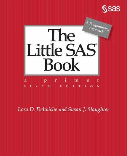
Example This example uses the permanent SAS data set created in Section 5.2. The data set contains the average lengths, in feet, of selected whales and sharks. The following program contains two procedures: PROC MEANS and PROC PRINT. There are three ODS statements in the program: one to open the LISTING destination, one to turn off procedure titles, and one to close the destination.
* Create the text output and remove procedure name;
LIBNAME ocean 'c:MySASLib';
ODS LISTING FILE = 'c:MyTextFilesMarine.lst';
ODS NOPROCTITLE;
PROC MEANS DATA = ocean.marine MEAN MIN MAX;
CLASS Family;
TITLE 'Whales and Sharks';
RUN;
PROC PRINT DATA = ocean.marine;
RUN;
ODS LISTING CLOSE;
Here is what the text file produced by SAS Enterprise Guide looks like when viewed in Microsoft Notepad. The LISTING destination does not use a style for tabular output. Instead, the results are rendered as plain text.
You may also be able to create text output without using ODS statements. The options available depend on the interface you use to run SAS. With a little exploration you, will find various menus and tasks for creating, exporting, and saving text output.
5.6 Customizing Titles and Footnotes
In ODS output, your style template tells SAS how titles and footnotes should look. However, you can easily change the appearance of titles and footnotes by inserting a few simple options in your TITLE and FOOTNOTE statements.
The general form for a TITLE or FOOTNOTE statement is:
TITLE options 'text-string-1' options 'text-string-2' ... options 'text-string-n';
FOOTNOTE options 'text-string-1' options 'text-string-2' ...options 'text-string-n';
Text can be broken into pieces with different options for each piece. SAS will concatenate text strings just the way you type them, so be sure to include any necessary blanks. Each option applies to the text string that follows, and stays in effect until another value is specified for that option, or until the end of the statement. Here are the main options that you can choose:
|
COLOR= |
specifies a color for the text |
|
BCOLOR= |
specifies a color for the background of the text |
|
HEIGHT= |
specifies the height of the text |
|
JUSTIFY= |
requests justification |
|
FONT= |
specifies a font for the text |
|
BOLD |
makes text bold |
|
ITALIC |
makes text italic |
Color The COLOR= option specifies the color of the text. This statement:
TITLE COLOR=BLACK 'Black ' COLOR=GRAY 'Gray ' COLOR=LTGRAY 'Light Gray';
produces this title:
Black Gray Light Gray |
SAS supports hundreds of colors ranging from primary colors—red—to more esoteric colors—LIGRPR (light grayish purplish red). These colors can be specified by name—BLUE—or by hexadecimal code—#0000FF. In fact, SAS recognizes more than a half-dozen naming schemes for specifying color. (For more information about colors, search for “SAS color-naming schemes” in the SAS Documentation or on the internet.) Names of colors need quotation marks if the name is longer than 8 characters or contains embedded spaces. RGB hexadecimal codes beginning with a pound sign also require quotation marks. If you want to specify colors by name, here is a list of basic colors that you can start with: AQUA, BLACK, BLUE, FUCHSIA, GREEN, GRAY, LIME, MAROON, NAVY, OLIVE, PURPLE, RED, SILVER, TEAL, WHITE, YELLOW.
Background color The BCOLOR= option specifies a background color. This statement uses an RGB hexadecimal code:
TITLE BCOLOR = '#C0C0C0' 'This Title Has a Gray Background';
and produces this title:
This Title Has a Gray Background |
You can choose among the same colors as with the COLOR= option.
Height To change the height of the text, use the HEIGHT= option where the value of HEIGHT is a number with units of PT, IN, or CM. This statement:
TITLE HEIGHT="12PT" 'Small ' HEIGHT=.25IN 'Medium ' HEIGHT="1CM" 'Large';
produces this title:
|
Small Medium Large |
Justification You can control justification of text using the JUSTIFY= option, which can have the values LEFT, CENTER, or RIGHT. You can even mix these options within a single statement. This statement:
TITLE JUSTIFY=LEFT 'Left ' JUSTIFY=CENTER 'vs. ' JUSTIFY=RIGHT 'Right';
produces this title:
|
Left |
vs. |
Right |
Font Use the FONT= option to specify a font. This statement:
TITLE 'Default ' FONT=Arial 'Arial '
FONT='Times New Roman' 'Times New Roman ' FONT=Courier 'Courier';
produces this title:
|
Default Arial Times New Roman Courier |
The particular fonts available to you depend on your operating environment and hardware. Courier, Arial, Times, and Helvetica work in most situations.
Bold and italic By default, titles are bold. When you change the font, you also turn off the bolding. To turn on bolding, use the BOLD option; to turn on italics use the ITALIC option. There is no option to turn off bolding or italics, so if you want to turn them off, use the FONT= option. Here are the three options together:
TITLE FONT = Courier 'Courier ' BOLD 'Courier Bold '
ITALIC 'Courier Bold and Italic';
This statement produces this title:
|
Courier Bold Courier Bold and Italic |
5.7 Customizing PROC PRINT with the STYLE= Option
If you want to change the overall look of any output, you can specify a different style template using a STYLE= option in your ODS statement. But what if you want to change the appearance of just the headers, or just one column of your output? With most procedures, you would need to use PROC TEMPLATE to create a custom style template. However, the reporting procedures, PRINT, REPORT, and TABULATE, allow you to change the style of various parts of the table using the STYLE= option in the procedures’ own statements.
The general form of the STYLE= option in the PROC PRINT statement is:
PROC PRINT STYLE(location-list) = {style-attribute = value};
where location-list specifies the parts of the table that should take on the style, style-attribute is the characteristic that you want to change, and value is the way you want the style attribute to look. (See Section 5.11 for a table of attributes and possible values.) For example, the following statement tells SAS to use a gray background for the data in the table.
PROC PRINT DATA = mysales STYLE(DATA) = {BACKGROUNDCOLOR = GRAY};
You can have several STYLE= options on one PROC PRINT statement, and the same style can apply to several locations. Here are some of the locations that you can specify:
|
Location |
Table region affected |
|
DATA |
all the data cells |
|
HEADER |
the column headers (variable names) |
|
OBS |
the data in the OBS column, or ID column if using an ID statement |
|
OBSHEADER |
the header for the OBS or ID column |
|
TOTAL |
the data in the totals row produced by a SUM statement |
|
GRANDTOTAL |
the data for the grand total produced by a SUM statement |
If you place the STYLE= option in the PROC PRINT statement, the entire table will be affected. For example, if you specify HEADER as the location, then all of the column headers will have the new style. To change the header of just one column, put the STYLE= option in the VAR statement:
VAR variable-list / STYLE(location-list) = {style-attribute = value};
Only the variables listed in the VAR statement will have the specified style. If you want different variables to have different styles, then use multiple VAR statements. Only the DATA and HEADER locations are valid on the VAR statement. You can apply styles to ID statements in the same way.
Example The following data are the top five finishers in the men’s 5000 meter speed skating event at the 2002 Winter Olympics. The skater’s place is followed by his name, country, and time in seconds.
Place,Name,Country,Time
1,Jochem Uytdehaage, Netherlands,374.66
2,Derek Parra, United States,377.98
3,Jens Boden, Germany,381.73
4,Dmitry Shepel, Russia,381.85
5,KC Boutiette, United States,382.97
This program creates a permanent SAS data set named RESULTS. Then a PROC PRINT uses the default destination and style template.
LIBNAME skate 'c:MySASLib';
PROC IMPORT DATAFILE = 'c:MyRawDataMens5000.csv' OUT = skate.results
REPLACE;
RUN;
PROC PRINT DATA = skate.results;
ID Place;
VAR Name Country Time;
TITLE "Men's 5000m Speed Skating";
RUN;
Here are the results:
Men's 5000m Speed Skating
|
Place |
Name |
Country |
Time |
|
1 |
Jochem Uytdehaage |
Netherlands |
374.66 |
|
2 |
Derek Parra |
United States |
377.98 |
|
3 |
Jens Boden |
Germany |
381.73 |
|
4 |
Dmitry Shepel |
Russia |
381.85 |
|
5 |
KC Boutiette |
United States |
382.97 |
The next program also uses the default style template, but the STYLE= option has been added to the PROC PRINT statement giving all the data cells a gray background and white foreground. A STYLE= option was also added to the ID statement to center the values of Place, and to a VAR statement making the values of Name italic.
* Use STYLE= option in PROC, ID, and VAR statements;
PROC PRINT DATA = skate.results
STYLE(DATA) = {BACKGROUNDCOLOR = GRAY COLOR = WHITE};
ID Place / STYLE(DATA) = {TEXTALIGN = CENTER};
VAR Name / STYLE(DATA) = {FONTSTYLE = ITALIC};
VAR Country Time;
TITLE "Men's 5000m Speed Skating";
RUN;
Here are the results:
Men’s 5000m Speed Skating
|
Place |
Name |
Country |
Time |
|
1 |
Jochem Uytdehaage |
Netherlands |
374.66 |
|
2 |
Derek Parra |
United States |
377.98 |
|
3 |
Jens Boden |
Germany |
381.73 |
|
4 |
Dmitry Shepel |
Russia |
381.85 |
|
5 |
KC Boutiette |
United States |
382.97 |
5.8 Customizing PROC REPORT with the STYLE= Option
With the STYLE= option in an ODS statement you can change the overall style of PROC REPORT output, but you can also use the STYLE= option inside PROC REPORT to change the style of individual features. The STYLE= option in PROC REPORT is similar to the PRINT procedure because you have to specify a location. The general form of the STYLE= option in the PROC REPORT statement is:
PROC REPORT STYLE(location-list) = {style-attribute = value};
where location-list specifies the parts of the table that should take on the style, style-attribute is the characteristic that you want to change, and value is the way you want the style attribute to look. (See Section 5.11 for a table of attributes and possible values.) For example, to give column headers a green background, you could use this statement:
PROC REPORT DATA = mysales STYLE(HEADER) = {BACKGROUNDCOLOR = GREEN};
You can specify more than one location in a single STYLE= option, and you can have several STYLE= options in one PROC REPORT statement. Here are some of the locations whose appearance you can control in PROC REPORT:
|
Location |
Table region affected |
|
HEADER |
column headings |
|
COLUMN |
data cells |
|
SUMMARY |
totals created by SUMMARIZE option in BREAK or RBREAK statements |
If you put a STYLE= option in a PROC REPORT statement, then it will affect the whole table, for example, all the column headings, all the data cells, or all the summary breaks. You can change part of a report by using the STYLE= option in other statements. To specify a style for a particular variable, put the STYLE= option in a DEFINE statement. If you use a GROUP or ORDER variable, you may want to add the SPANROWS option to the PROC statement. The SPANROWS option combines cells in the same category into a single cell. These statements tell SAS to use Month as a group variable, and make the background blue for both the header and the data:
PROC REPORT DATA = mysales SPANROWS;
DEFINE Month / GROUP STYLE(HEADER COLUMN) = {BACKGROUNDCOLOR = BLUE};
To specify a style for particular summary breaks, use the STYLE= option in a BREAK or RBREAK statement. This statement tells SAS to use a red background for summary breaks for each value of Month.
BREAK AFTER Month / SUMMARIZE STYLE(SUMMARY) = {BACKGROUNDCOLOR = RED};
Example This example uses the permanent SAS data set created in the preceding section. The data are the top five finishers in the men’s 5000 meter speed skating event at the 2002 Winter Olympics. The variables are each skater’s place, name, country, and time in seconds.
This program uses the default destination and style template:
LIBNAME skate 'c:MySASLib';
PROC REPORT DATA = skate.results;
COLUMN Country Name Time Place;
DEFINE Country / ORDER;
TITLE "Men's 5000m Speed Skating";
RUN;
Here are the results:
Men’s 5000m Speed Skating
|
Country |
Name |
Time |
Place |
|
Germany |
Jens Boden |
381.73 |
3 |
|
Netherlands |
Jochem Uytdehaage |
374.66 |
1 |
|
Russia |
Dmitry Shepel |
381.85 |
4 |
|
United States |
Derek Parra |
377.98 |
2 |
|
|
KC Boutiette |
382.97 |
5 |
The next program also uses the default style template, but it adds a STYLE= option in the PROC REPORT statement to change the background of all the data cells to gray and the foreground text to white. Then it adds the STYLE= option in the DEFINE statements to italicize the values of Name and to center the values of Place. The SPANROWS option combines the two lines for the United States into one cell.
* Use STYLE= option in PROC and DEFINE statements;
PROC REPORT DATA = skate.results SPANROWS
STYLE(COLUMN) = {BACKGROUNDCOLOR = GRAY COLOR = WHITE};
COLUMN Country Name Time Place;
DEFINE Country / ORDER;
DEFINE Name / STYLE(COLUMN) = {FONTSTYLE = ITALIC};
DEFINE Place / STYLE(COLUMN) = {TEXTALIGN = CENTER};
TITLE "Men's 5000m Speed Skating";
RUN;
Here are the results:
Men's 5000m Speed Skating
|
Country |
Name |
Time |
Place |
|
Germany |
Jens Boden |
381.73 |
3 |
|
Netherlands |
Jochem Uytdehaage |
374.66 |
1 |
|
Russia |
Dmitry Shepel |
381.85 |
4 |
|
United States |
Derek Parra |
377.98 |
2 |
|
KC Boutiette |
382.97 |
5 |
5.9 Customizing PROC TABULATE with the STYLE= Option
Like the PRINT and REPORT procedures, PROC TABULATE allows you to control the style of individual features with the STYLE= option. However, unlike PROC PRINT and PROC REPORT, you do not have to specify a location. The part of the table affected depends on where you place the STYLE= option. (See Section 5.11 for a table of style attributes and their possible values.) Here are some of the PROC TABULATE statements that accept the STYLE= option:
|
Statement |
Table region affected |
|
PROC TABULATE |
all the data cells |
|
CLASS |
class variable name headings |
|
CLASSLEV |
class level value headings |
|
TABLE (crossed with elements) |
element’s data cell |
|
VAR |
analysis variable name headings |
PROC TABULATE statement If you place the STYLE= option in the PROC TABULATE statement, all the table’s data cells will have the style. For example, if you wanted all the data cells in your table created from the MYSALES SAS data set to have a yellow background, then you would use the following statement:
PROC TABULATE DATA = mysales STYLE = {BACKGROUNDCOLOR = YELLOW};
TABLE statement If you want some of the data cells to have a different style from the rest, then you need to add the STYLE= option to the TABLE statement and cross the style with the variable or keyword you want to change (similar to having different formats for different parts of the table, as discussed in Section 4.17). Any style assigned in a TABLE statement will override styles assigned in the PROC TABULATE statement. For example, the following TABLE statement produces a table where the data cells in the ALL column have a red background:
TABLE City, Month ALL*{STYLE = {BACKGROUNDCOLOR = RED}};
CLASSLEV, VAR, and CLASS statements The CLASSLEV, VAR, and CLASS statements all require that you place the STYLE= option after a slash (/). Any variable that appears in a CLASSLEV statement must also appear in a CLASS statement. For example, suppose that you had a table with a class variable Month, and you wanted all the values of Month to have a foreground color of green, then you would use this CLASSLEV statement:
CLASSLEV Month / STYLE = {COLOR = GREEN};
Example This example uses the permanent SAS data set created in Section 5.2. The data set contains the average lengths, in feet, of selected whales and sharks.
This program uses the default destination and style template:
LIBNAME ocean 'c:MySASLib';
PROC TABULATE DATA = ocean.marine;
CLASS Family;
VAR Length;
TABLE Family, Length*(Min Max Mean);
TITLE 'Whales and Sharks';
RUN;
Here are the results:
Whales and Sharks
|
|
Length |
||
|
Min |
Max |
Mean |
|
|
Family |
0.50 |
40.00 |
20.63 |
|
shark |
|||
|
whale |
15.00 |
100.00 |
48.75 |
The next program uses the default style template, but adds a STYLE= option to the PROC statement giving the data cells white foreground text and a gray background. Then the STYLE= options in the CLASS and VAR statements apply an italic style to the headings for those variables.
* Use STYLE= option in PROC, CLASS, and VAR statements;
PROC TABULATE DATA = ocean.marine
STYLE = {BACKGROUNDCOLOR = GRAY COLOR = WHITE};
CLASS Family / STYLE = {FONTSTYLE = ITALIC};
VAR Length / STYLE = {FONTSTYLE = ITALIC};
TABLE Family, Length*(Min Max Mean);
TITLE 'Whales and Sharks';
RUN;
Here are the results:
Whales and Sharks
|
|
Length |
||
|
Min |
Max |
Mean |
|
|
Family |
0.50 |
40.00 |
20.63 |
|
shark |
|||
|
whale |
15.00 |
100.00 |
48.75 |
5.10 Adding Trafficlighting to Your Output
![]()
Trafficlighting is a feature that allows you to control the style of cells in the table based on the values of the data in the cells. This way you can draw attention to important values in your report, or highlight relationships between values. Trafficlighting can be used in any of the three reporting procedures: PRINT, REPORT, and TABULATE.
To implement trafficlighting you need to do two things. First, create a user-defined format where the ranges of data values correspond to different values of a style attribute. (See the following section for a table of style attributes and their possible values.) Next, set the style attribute equal to your user-defined format in a STYLE= option. For example, you could create this format:
PROC FORMAT;
VALUE posneg
LOW -< 0 = 'RED'
0-HIGH = 'BLACK';
RUN;
Then with a VAR statement in a PRINT procedure, you could set the value of the COLOR attribute equal to your user-defined format (POSNEG.), like this:
VAR Balance / STYLE = {COLOR = posneg.};
Then all the data cells for the variable Balance would have red numbers if they are negative and black numbers if they are positive.
Example This example uses the permanent SAS data set created in Section 5.7. The data are the top five finishers in the men’s 5000 meter speed skating event at the 2002 Winter Olympics. The skater’s place is followed by his name, country, and time in seconds.
The following program prints the data using PROC PRINT. The resulting output uses the default destination and the default style.
LIBNAME skate 'c:MySASLib';
PROC PRINT DATA = skate.results;
ID Place;
TITLE "Men's 5000m Speed Skating";
RUN;
Here are the results:
Men's 5000m Speed Skating
|
Place |
Name |
Country |
Time |
|
1 |
Jochem Uytdehaage |
Netherlands |
374.66 |
|
2 |
Derek Parra |
United States |
377.98 |
|
3 |
Jens Boden |
Germany |
381.73 |
|
4 |
Dmitry Shepel |
Russia |
381.85 |
|
5 |
KC Boutiette |
United States |
382.97 |
We can use trafficlighting to give an idea of how these times compare with previous times for this event. Prior to the 2002 Olympics, the world record for the 5000 meter speed skating was 378.72 seconds and the Olympic record was 382.20 seconds. To show which skaters skated faster than these records, the following PROC FORMAT creates a user-defined format, named REC., which assigns the color light gray to times less than the world record, very light gray to times less than the Olympic record, and white to other times. The second VAR statement in the PROC PRINT uses the STYLE= option to set the BACKGROUNDCOLOR attribute of the values for the variable Time equal to the REC. format.
* Create user-defined format for colors;
PROC FORMAT;
VALUE rec 0 -< 378.72 = 'LIGHT GRAY'
378.72 -< 382.20 = 'VERY LIGHT GRAY'
382.20 - HIGH = 'WHITE';
RUN;
* Use STYLE= option to apply format in VAR statement;
PROC PRINT DATA = skate.results;
ID Place;
VAR Name Country;
VAR Time / STYLE = {BACKGROUNDCOLOR = rec.};
TITLE "Men's 5000m Speed Skating";
RUN;
Here is the output showing the different colored backgrounds based on the value of Time. Those skaters who broke the previous world record have a light gray background for Time, those who broke the Olympic record have a very light gray background, and the fifth skater who didn’t break any records has a white background.
Men's 5000m Speed Skating
|
Place |
Name |
Country |
Time |
|
1 |
Jochem Uytdehaage |
Netherlands |
374.66 |
|
2 |
Derek Parra |
United States |
377.98 |
|
3 |
Jens Boden |
Germany |
381.73 |
|
4 |
Dmitry Shepel |
Russia |
381.85 |
|
5 |
KC Boutiette |
United States |
382.97 |
5.11 Selected Style Attributes
|
Attribute |
Description |
Possible Values |
|
BACKGROUNDCOLOR or BACKGROUND |
Specifies the background color of the table or cell. |
Any valid color 1 |
|
BACKGROUNDIMAGE |
Specifies a background image to be used for the table or cell. Not valid for RTF. |
Any GIF, JPEG, or PNG image file 2 |
|
COLOR or FOREGROUND |
Specifies the color of the text in the cells. |
Any valid color 1 |
|
FLYOVER |
Specifies the pop-up text displayed when the cursor is held over the text (HTML) or if you double-click on the text (PDF). |
Any text string enclosed in quotation marks |
|
FONTFAMILY or FONT_FACE |
Specifies the font to use for the text in the cells. |
Any valid font (Most devices support Times, Courier, Arial, and Helvetica) |
|
FONTSIZE or FONT_SIZE |
Specifies the relative size of the font for the text in cells.3 |
1 to 7 |
|
FONTSTYLE or FONT_STYLE |
Specifies the style of the font used in the cells. |
ITALIC, ROMAN, or SLANT (Italic and slant may map to the same font) |
|
FONTWEIGHT or FONT_WEIGHT |
Specifies the weight of the font used in the cells. |
BOLD, MEDIUM, or LIGHT |
|
PREIMAGE or POSTIMAGE |
Specifies an image that will be inserted either before (PREIMAGE) or after (POSTIMAGE) the text in the cells. |
Any GIF, JPEG, or PNG image file (JPEG and PNG only for RTF) 2 |
|
PRETEXT or POSTTEXT |
Specifies text that goes either before (PRETEXT) or after (POSTTEXT) the text in the cells. |
Any text string enclosed in quotation marks |
|
TEXTALIGN or JUST |
Specifies the justification of the text in the cells. |
R|RIGHT, C|CENTER, L|LEFT, or D (decimal) |
|
URL |
Specifies the URL to link to from the text in the cell. HTML, PDF, and RTF only. |
Any URL |
1 You can specify colors by name including AQUA, BLACK, BLUE, FUCHSIA, GREEN, GRAY, LIME, MAROON, NAVY, OLIVE, PURPLE, RED, SILVER, TEAL, WHITE, and YELLOW. For an exact color you can use the RGB notation such as #00FF00 for green. To learn more, search for “SAS color-naming schemes” in the SAS Documentation or on the internet.
2 For HTML, if you use a simple filename, then the SAS internal browser may not be able to find the file. If you use a complete path and then move the files to a new location, be sure to edit the HTML file to reflect the new location.
3 For some destinations, you can specify size in units of measure: cm, in, mm, pt, px (pixels). For example, if you want text that is 24 points, then you would specify FONTSIZE=24pt.
|
Attribute |
STYLE= code |
Result |
|
BACKGROUNDCOLOR or BACKGROUND |
STYLE(DATA)= {BACKGROUNDCOLOR=WHITE}; |
|
|
BACKGROUNDIMAGE |
STYLE(DATA)= {BACKGROUNDIMAGE= 'c:MyImagessnow.gif'}; |
|
|
COLOR or FOREGROUND |
STYLE(DATA)= {COLOR=WHITE}; |
|
|
FLYOVER |
STYLE(DATA)= {FLYOVER='Try it!'}; |
|
|
FONTFAMILY or FONT_FACE |
STYLE(DATA)= {FONTFAMILY=COURIER}; |
|
|
FONTSIZE or FONT_SIZE |
STYLE(DATA)= {FONTSIZE=2}; |
|
|
FONTSTYLE or FONT_STYLE |
STYLE(DATA)= {FONTSTYLE=ITALIC}; |
|
|
FONTWEIGHT or FONT_WEIGHT |
STYLE(DATA)= {FONTWEIGHT=BOLD}; |
|
|
PREIMAGE or POSTIMAGE |
STYLE(DATA)= {PREIMAGE='SS2.gif'}; |
|
|
PRETEXT or POSTTEXT |
STYLE(DATA)= {POSTTEXT=' is fun'}; |
|
|
TEXTALIGN or JUST |
STYLE(DATA)= {TEXTALIGN=RIGHT}; |
|
|
URL |
STYLE(DATA)= {URL='http://skating.org'}; |
|
5.12 Tracing and Selecting Procedure Output

When ODS receives data from a procedure, it combines the data with a table template. Together the data and corresponding table template are called an output object. Many procedures produce just one output object, while others produce several. For most procedures, when you use a BY statement, SAS produces one output object for each BY group. Every output object has a name. You can find the names of output objects by using the ODS TRACE statement. Then you can use an ODS SELECT (or ODS EXCLUDE) statement to choose just the output objects that you want.
ODS TRACE statement The ODS TRACE statement tells SAS to print information about output objects in your SAS log. There are two ODS TRACE statements: one to turn on the trace, and one to turn it off. Here is how to use these statements in a program:
ODS TRACE ON;
the PROC steps you want to trace go here
RUN;
ODS TRACE OFF;
Notice that the RUN statement comes before the ODS TRACE OFF statement. Unlike most other SAS statements, ODS statements execute immediately—without waiting for a RUN, PROC, or DATA statement. If you put the ODS TRACE OFF statement before the RUN statement, then the trace would turn off before the procedure completes.
Example Here are data about varieties of giant tomatoes. Each line of data includes the name of the variety, its color (red or yellow), the number of days from planting to harvest, and the weight (in pounds) of a typical tomato. Each line of data includes two varieties.
Big Zac, red, 80, 5, Delicious, red, 80, 3
Dinner Plate, red, 90, 2, Goliath, red, 85, 1.5
Mega Tom, red, 80, 2, Mortgage Lifter, red, 85, 2
Big Rainbow, yellow, 90, 1.5, Pineapple, yellow, 85, 2
The following program creates a permanent SAS data set named GIANT, and then traces PROC MEANS using ODS TRACE ON and ODS TRACE OFF statements:
LIBNAME tomatoes 'c:MySASLib';
DATA tomatoes.giant;
INFILE 'c:MyRawDataGiantTom.dat' DSD;
INPUT Name :$15. Color $ Days Weight @@;
RUN;
* Trace PROC MEANS;
ODS TRACE ON;
PROC MEANS DATA = tomatoes.giant;
BY Color;
RUN;
ODS TRACE OFF;
If you run this program, you will see the following trace in your SAS log. Because it contains a BY statement, the MEANS procedure produces one output object for each BY group (red and yellow). Notice that these two output objects have the same name, label, and template, but different paths.
Output Added:
-------------
Name: Summary
Label: Summary statistics
Template: base.summary
Path: Means.ByGroup1.Summary
-------------
NOTE: The above message was for the following BY group: Color=red
Output Added:
-------------
Name: Summary
Label: Summary statistics
Template: base.summary
Path: Means.ByGroup2.Summary
-------------
NOTE: The above message was for the following BY group: Color=yellow
ODS SELECT statement Once you know the names of the output objects that the procedure uses, you can use an ODS SELECT (or EXCLUDE) statement to choose just the output objects you want. The general form of an ODS SELECT statement is:
The PROC step with the output objects you want to select
ODS SELECT output-object-list;
RUN;
where output-object-list is the name, label, or path of one or more output objects separated by spaces. By default, an ODS SELECT statement lasts for only one PROC step, so by placing the SELECT statement after the PROC statement and before the RUN statement, you are sure to capture the correct output. ODS EXCLUDE statements work the same way except you list output objects that you want to eliminate.
Example This program runs PROC MEANS again using the GIANT data set, and an ODS SELECT statement to select just the first output object: Means.ByGroup1.Summary.
* Print only the first BY group;
PROC MEANS DATA = tomatoes.giant;
BY Color;
ODS SELECT Means.ByGroup1.Summary;
RUN;
Here are the results containing just the first BY group:
|
The MEANS Procedure |
Color=red
|
Variable |
N |
Mean |
Std Dev |
Minimum |
Maximum |
|
Days |
6 |
83.3333333 |
4.0824829 |
80.0000000 |
90.0000000 |
5.13 Creating SAS Data Sets from Procedure Output

Sometimes you may want to put the results from a procedure into a SAS data set. Once the results are in a data set, you can merge them with another data set, compute new variables based on the results, or use the results as input for other procedures. Some procedures have OUTPUT statements, or OUT= options, allowing you to save the results as a SAS data set. But with ODS you can save almost any part of procedure output as a SAS data set by sending it to the OUTPUT destination. First you use an ODS TRACE statement (discussed in the previous section) to determine the name of the output object you want. Then you use an ODS OUTPUT statement to send that object to the OUTPUT destination.
ODS OUTPUT statement Here is the general form of a basic ODS OUTPUT statement:
ODS OUTPUT output-object = new-data-set;
where output-object is the name, label, or path of the piece of output you want to save, and new-data-set is the name of the SAS data set you want to create.
The ODS OUTPUT statement does not belong to either a DATA or PROC step, but you need to be careful where you put it in your program. The ODS OUTPUT statement opens a SAS data set and waits for the correct procedure output. The data set remains open until the next encounter with the end of a PROC step. Because the ODS OUTPUT statement executes immediately, it will apply to whatever PROC is currently being processed, or it will apply to the next PROC if there is not a current PROC. To ensure that you get the correct output, it is a good idea to put the ODS OUTPUT statement after your PROC statement, and before the next PROC, DATA, or RUN statement.
Example This example uses the permanent SAS data set created in the preceding section. The data set contains information about varieties of giant tomatoes including the name of the variety, its color (red or yellow), the number of days from planting to harvest, and the weight (in pounds) of a typical tomato.
To find the name of the desired output object, the following program traces PROC TABULATE using ODS TRACE ON and ODS TRACE OFF statements:
LIBNAME tomatoes 'c:MySASLib';
ODS TRACE ON;
PROC TABULATE DATA = tomatoes.giant;
CLASS Color;
VAR Days Weight;
TABLE Color ALL, (Days Weight) * MEAN;
RUN;
ODS TRACE OFF;
Here is an excerpt from the SAS log showing the trace produced by PROC TABULATE. PROC TABULATE produces one output object named Table. The names of output objects do not change so you can skip this step if you already know the name of the output object you want to capture.
Output Added:
-------------
Name: Table
Label: Table 1
Data Name: Report
Path: Tabulate.Report.Table
-------------
The following program uses an ODS OUTPUT statement to create a temporary SAS data set named TABOUT from the Table output object.
PROC TABULATE DATA = tomatoes.giant;
CLASS Color;
VAR Days Weight;
TABLE Color ALL, (Days Weight) * MEAN;
TITLE 'Standard TABULATE Output';
ODS OUTPUT Table = tabout;
RUN;
Here is the standard tabular result produced by PROC TABULATE:
Standard TABULATE Output
|
|
Days |
Weight |
|
Mean |
Mean |
|
|
Color |
83.33 |
2.58 |
|
red |
||
|
yellow |
87.50 |
1.75 |
|
All |
84.38 |
2.38 |
Here is the TABOUT data set created by the ODS OUTPUT statement:
|
|
Color |
_TYPE_ |
_PAGE_ |
_TABLE_ |
Days_Mean |
Weight_Mean |
|
1 |
red |
1 |
1 |
1 |
83.3333 |
2.58333 |
|
2 |
yellow |
1 |
1 |
1 |
87.5000 |
1.75000 |
|
3 |
|
0 |
1 |
1 |
84.3750 |
2.37500 |