CHAPTER 6

Modifying and Combining SAS Data Sets

6.1    Stacking Data Sets Using the SET Statement

6.2    Interleaving Data Sets Using the SET Statement

6.3    Combining Data Sets Using a One-to-One Match Merge

6.4    Combining Data Sets Using a One-to-Many Match Merge

6.5    Using PROC SQL to Join Data Sets

6.6     Merging Summary Statistics with the Original Data

6.7    Combining a Grand Total with the Original Data

6.8    Adding Summary Statistics to Data Using PROC SQL

6.9    Updating a Master Data Set with Transactions

6.10  Using SAS Data Set Options

6.11  Tracking and Selecting Observations with the IN= Option

6.12  Selecting Observations with the WHERE= Option

6.13  Changing Observations to Variables Using PROC TRANSPOSE

6.14  Using SAS Automatic Variables

6.1     Stacking Data Sets Using the SET Statement

So far in the book, you have seen many examples of using a SET statement to read a single data set. You can also use SET statements to concatenate or stack data sets. This is useful when you want to combine data sets with all or most of the same variables but different observations. For example, you might have data from two different locations or data taken at two separate times, but you need the data together for analysis.

In a DATA step, first specify the name of the new SAS data set in the DATA statement, then list the names of the old data sets you want to combine in the SET statement.

             DATA new-data-set;

                SET data-set-1 data-set-n;

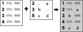
The number of observations in the new data set will equal the sum of the number of observations in the old data sets. The order of observations is determined by the order of the list of old data sets. If one of the data sets has a variable not contained in the other data sets, then the observations from the other data sets will have missing values for that variable.

Example  The Fun Times Amusement Park has two entrances where they collect data about their customers. The data file for the south entrance has an S (for south) followed by the customers’ Fun Times pass numbers, the sizes of their parties, and their ages. The file for the north entrance has an N (for north), the same data as the south entrance, plus one more variable for the parking lot where they left their cars (the south entrance has only one lot). The following shows samples of the two data files.

Data for the South entrance:

Entrance,PassNumber,PartySize,Age

S,43,3,27

S,44,3,24

S,45,3,2

Data for the North entrance:

Entrance,PassNumber,PartySize,Age,Lot

N,21,5,41,1

N,87,4,33,3

N,65,2,67,1

N,66,2,7,1

The first two parts of the following program read the comma-delimited data for the south and north entrances into SAS data sets using PROC IMPORT. The third part combines the two SAS data sets using a SET statement. The same DATA step creates a new variable, AmountPaid, which tells how much each customer paid based on their age:

PROC IMPORT DATAFILE = 'c:MyRawDataSouth.csv' OUT = southent REPLACE;

PROC IMPORT DATAFILE = 'c:MyRawDataNorth.csv' OUT = northent REPLACE;

RUN;

* Create a data set, both, combining northent and southent;

* Create a variable, AmountPaid, based on value of variable Age;

DATA both;

   SET southent northent;

   IF Age = . THEN AmountPaid = .;

      ELSE IF Age < 3  THEN AmountPaid = 0;

      ELSE IF Age < 65 THEN AmountPaid = 35;

      ELSE AmountPaid = 27;

RUN;

 Here is the SOUTHENT data set:

	Entrance	PassNumber	PartySize	Age
1	S	43	3	27
2	S	44	3	24
3	S	45	3	2

Here is the NORTHENT data set:

	Entrance	PassNumber	PartySize	Age	Lot
1	N	21	5	41	1
2	N	87	4	33	3
3	N	65	2	67	1
4	N	66	2	7	1

And here is the final data set, BOTH. Notice that this data set has missing values for the variable Lot for all the observations from the south entrance. Because the variable Lot was not in the SOUTHENT data set, SAS assigned missing values to those observations.

	Entrance	PassNumber	PartySize	Age	Lot	AmountPaid
1	S	43	3	27	.	35
2	S	44	3	24	.	35
3	S	45	3	2	.	0
4	N	21	5	41	1	35
5	N	87	4	33	3	35
6	N	65	2	67	1	27
7	N	66	2	7	1	35

The following notes appear in the SAS log stating that three observations were read from SOUTHENT, four observations from NORTHENT, and the final data set, BOTH, has seven observations. It is always a good idea to look at the SAS log and make sure that the number of observations and variables in the data sets makes sense.

NOTE: There were 4 observations read from the data set WORK.NORTHENT.

 

6.2    Interleaving Data Sets Using the SET Statement

The previous section explained how to stack data sets that have all or most of the same variables but different observations. However, if you have data sets that are already sorted by some important variable, then simply stacking the data sets may unsort the data sets. You could stack the two data sets and then re-sort them using PROC SORT. But if your data sets are already sorted, it is more efficient to preserve that order than to stack and re-sort. All you need to do is use a BY statement with your SET statement. Here’s the general form:

  DATA new-data-set;

     SET data-set-1 data-set-n;

                BY variable-list;

In a DATA statement, you specify the name of the new SAS data set you want to create. In a SET statement, you list the data sets to be interleaved. Then in a BY statement, you list one or more variables that SAS should use for ordering the observations. The number of observations in the new data set will be equal to the sum of the number of observations in the old data sets. If one of the data sets has a variable that is not contained in the other data sets, then the values of that variable will be set to missing for observations from the other data sets.

Before you can interleave observations, the data sets must be sorted by the BY variables. If one or the other of your data sets is not already sorted, then use PROC SORT to do the job.

Example  To show how this is different from stacking data sets, we’ll use the amusement park data again. There are two comma-separated data files, one for the south entrance and one for the north. For every customer, the park collects the following data: the entrance (S or N), the customer’s Fun Times pass number, size of that customer’s party, and age. For customers entering from the north, the data set also includes parking lot number. Notice that the data for the south entrance are already sorted by pass number, but the data for the north entrance are not.

Data for the South entrance:

Entrance,PassNumber,PartySize,Age

S,43,3,27

S,44,3,24

S,45,3,2

Data for the North entrance:

Entrance,PassNumber,PartySize,Age,Lot

N,21,5,41,1

N,87,4,33,3

N,65,2,67,1

N,66,2,7,1

Instead of stacking the two data sets, this program interleaves the data sets by pass number. This program first reads the data for the south entrance and north entrance using PROC IMPORT. Then the program sorts the north entrance data. In the final DATA step, SAS combines the two data sets, SOUTHENT and NORTHENT, creating a new data set named INTERLEAVE. The BY statement tells SAS to combine the data sets by PassNumber:

PROC IMPORT DATAFILE = 'c:MyRawDataSouth.csv' OUT = southent REPLACE;

PROC IMPORT DATAFILE = 'c:MyRawDataNorth.csv' OUT = northent REPLACE;

RUN;

PROC SORT DATA = northent;

   BY PassNumber;

RUN;

* Interleave observations by PassNumber;

DATA interleave;

   SET southent northent;

   BY PassNumber;

RUN;

Here is the SOUTHENT data set:

	Entrance	PassNumber	PartySize	Age
1	S	43	3	27
2	S	44	3	24
3	S	45	3	2

Here is the NORTHENT data set after sorting by PASSNUMBER:

	Entrance	PassNumber	PartySize	Age	Lot
1	N	21	5	41	1
2	N	65	2	67	1
3	N	66	2	7	1
4	N	87	4	33	3

And here is the data set named INTERLEAVE. Notice that the observations have been interleaved so that the final data set is sorted by PassNumber:

	Entrance	PassNumber	PartySize	Age	Lot
1	N	21	5	41	1
2	S	43	3	27	.
3	S	44	3	24	.
4	S	45	3	2	.
5	N	65	2	67	1
6	N	66	2	7	1
7	N	87	4	33	3

The following notes appear in the SAS log stating that three observations were read from SOUTHENT, four observations from NORTHENT, and the final data set, INTERLEAVE, has seven observations. It is always a good idea to look at the SAS log and make sure that the number of observations and variables in the data sets makes sense.

NOTE: There were 4 observations read from the data set WORK.NORTHENT.

6.3     Combining Data Sets Using a One-to-One Match Merge

When you want to match observations from one data set with observations from another, you can use the MERGE statement in the DATA step. If you know the two data sets are in EXACTLY the same order, you don’t have to have any common variables between the data sets. Typically, however, you will want to have, for matching purposes, a common variable or several variables which taken together uniquely identify each observation. This is important. Having a common variable to merge by ensures that the observations are properly matched. For example, to merge patient data with billing data, you would use the patient ID as a matching variable. Otherwise, you risk getting Mary Smith’s visit to the obstetrician mixed up with Matthew Smith’s visit to the optometrist.

Merging SAS data sets is a simple process. First, if the data are not already sorted, use the SORT procedure to sort all data sets by the common variables. Then, in the DATA statement, name the new SAS data set to hold the results and follow with a MERGE statement listing the data sets to be combined. Use a BY statement to indicate the common variables:

DATA new-data-set;

   MERGE data-set-1 data-set-n;

   BY variable-list;

If you merge two data sets, and they have variables with the same names—besides the BY variables—then variables from the second data set will overwrite any variables that have the same name in the first data set.

Example  A Belgian chocolatier keeps track of the number of each type of chocolate sold each day. The code for each chocolate and the number of pieces sold that day are kept in a file. In a separate file she keeps the names and descriptions of each chocolate as well as the code. In order to print the day’s sales along with the descriptions of the chocolates, the two files must be merged together using the code as the common variable. Here is a sample of the data:

Sales data                        Descriptions data

Code   Sold        Code   Name        Description

C865   15          A206   Mokka       Coffee buttercream in dark chocolate

K086   9           A536   Walnoot     Walnut halves in dark chocolate

A536   21          B713   Frambozen   Raspberry marzipan in milk chocolate

S163   34          C865   Vanille     Vanilla-flavored rolled in hazelnuts

K014   1           K014   Kroon       Milk chocolate with mint cream

A206   12          K086   Koning      Hazelnut paste in dark chocolate

B713   29          M315   Pyramide    White with dark chocolate trimming

                   S163   Orbais      Chocolate cream in dark chocolate

 

The first two parts of the following program read the tab-delimited files for the descriptions and sales data using PROC IMPORT. The descriptions data are already sorted by Code, so we don’t need to use PROC SORT. The sales data are not sorted, so a PROC SORT follows the PROC IMPORT step for the SALES data set. (If you attempt to merge data that are not sorted, SAS will refuse and give you this error message: ERROR: BY variables are not properly sorted.)

PROC IMPORT DATAFILE = 'c:MyRawDataChocolate.txt' OUT = names REPLACE;

PROC IMPORT DATAFILE = 'c:MyRawDataChocsales.txt' OUT = sales REPLACE;

RUN;

PROC SORT DATA = sales;

   BY Code;

RUN;

* Merge data sets by Code;

DATA chocolates;

   MERGE sales names;

   BY Code;

RUN;

The final part of the program creates a data set named CHOCOLATES by merging the SALES data set and the NAMES data set. The common variable Code in the BY statement is used for matching purposes. Here is the final data set after merging:

	Code	Sold	Name	Description
1	A206	12	Mokka	Coffee buttercream in dark chocolate
2	A536	21	Walnoot	Walnut halves in dark chocolate
3	B713	29	Frambozen	Raspberry marzipan in milk chocolate
4	C865	15	Vanille	Vanilla-flavored rolled in hazelnuts
5	K014	1	Kroon	Milk chocolate with mint cream
6	K086	9	Koning	Hazelnut paste in dark chocolate
7	M315	.	Pyramide	White with dark chocolate trimming
8	S163	34	Orbais	Chocolate cream in dark chocolate

Notice that the final data set has a missing value for Sold in the seventh observation. This is because there were no sales for the Pyramide chocolate. All observations from both data sets were included in the final data set whether they had a match or not. In SQL terms, this is called a full outer join. SAS can do all types of joins using the IN= option (Section 6.11), or PROC SQL (Section 6.5).

The following notes appear in the SAS log stating that seven observations were read from SALES, eight observations from NAMES, and the final data set, CHOCOLATES, has eight observations. It is always a good idea to look at the SAS log and make sure that the number of observations and variables in the data sets makes sense.

NOTE: There were 8 observations read from the data set WORK.NAMES.

 

6.4      Combining Data Sets Using a One-to-Many Match Merge

Sometimes you need to combine two data sets by matching one observation from one data set with more than one observation in another. Suppose you had data for every state in the U.S. and wanted to combine it with data for every county. This would be a one-to-many match merge because each state observation matches with many county observations.

The statements for a one-to-many match merge are identical to the statements for a one-to-one match merge:

DATA new-data-set;

   MERGE data-set-1 data-set-2;

   BY variable-list;

The order of the data sets in the MERGE statement does not affect the matching. In other words, a one-to-many merge will match the same observations as a many-to-one merge.

Before you merge two data sets, they must be sorted by one or more common variables. If your data sets are not already sorted in the proper order, then use PROC SORT to do the job.

You cannot do a one-to-many merge without a BY statement. SAS uses the variables listed in the BY statement to decide which observations belong together. Without a BY statement, SAS simply joins together the first observation from each data set, then the second observation from each data set, and so on. In other words, SAS performs a one-to-one unmatched merge, which is probably not what you want.

If you merge two data sets, and they contain variables with the same name—besides the BY variables—then you should either rename the variables or drop one of the duplicate variables. Otherwise, variables from the second data set may overwrite variables having the same name in the first data set. For example, if you merge two data sets that each contain a variable named BirthDate, then you could rename the variables (perhaps as BirthDate1 and BirthDate2), or you could simply drop BirthDate from one data set. Then the values of BirthDate will not overwrite each other. You can use the RENAME= and DROP= data set options (discussed in Section 6.10) to prevent the overwriting of data values.

Example  A distributor of athletic shoes is putting all its shoes on sale at 15% to 30% off the regular price. The distributor has two data files, one with information about each type of shoe and one with the discount factors. The first file contains one record for each shoe with values for style, type of exercise (basketball, running, walking, or cross-training), and regular price. The second file contains one record for each type of exercise and its discount. Here are the two raw data files:

Shoes data                                                           Discount data

Max Flight      running 142.99     b-ball  .15

Zip Fit Leather walking  83.99     c-train .25

Zoom Airborne   running 112.99     running .30

Light Step      walking  73.99     walking .20

Max Step Woven  walking  75.99

Zip Sneak       c-train  92.99

To find the sale price, the following program combines the two data files:

LIBNAME athshoes 'c:MySASLib';

DATA athshoes.shoedata;

   INFILE 'c:MyRawDataShoe.dat';

   INPUT Style $ 1-15 ExerciseType $ RegularPrice;

RUN;

PROC SORT DATA = athshoes.shoedata OUT = regular;

   BY ExerciseType;

RUN;

DATA athshoes.discount;

   INFILE 'c:MyRawDataDisc.dat';

   INPUT ExerciseType $ Adjustment;

RUN;

* Perform many-to-one match merge;

DATA prices;

   MERGE regular athshoes.discount;

   BY ExerciseType;

   NewPrice = ROUND(RegularPrice - (RegularPrice * Adjustment), .01);

RUN;

The first DATA step reads the shoes data into a SAS data set, then PROC SORT sorts the data by ExerciseType and creates a new temporary data set named REGULAR. The second DATA step reads the price adjustments, creating a permanent data set named DISCOUNT. This data set is already arranged by ExerciseType, so it doesn’t have to be sorted. The third DATA step creates a data set named PRICES, merging the first two data sets by ExerciseType, and computes a variable called NewPrice. The final data set looks like this:

	Style	ExerciseType	RegularPrice	Adjustment	NewPrice
1		b-ball	.	0.15	.
2	Zip Sneak	c-train	92.99	0.25	69.74
3	Max Flight	running	142.99	0.30	100.09
4	Zoom Airborne	running	112.99	0.30	79.09
5	Zip Fit Leather	walking	83.99	0.20	67.19
6	Light Step	walking	73.99	0.20	59.19
7	Max Step Woven	walking	75.99	0.20	60.79

Notice that the values for Adjustment from the DISCOUNT data set are repeated for every observation in the REGULAR data set with the same value of ExerciseType. Also, the first observation contains missing values for variables from the REGULAR data set. All observations from both data sets were included in the final data set whether they had a match or not. In SQL, this is called a full outer join. SAS can do all types of joins using the IN= option (Section 6.11) or PROC SQL (Section 6.5).

The following notes appear in the SAS log stating that six observations were read from REGULAR, four observations from DISCOUNT, and the final data set, PRICES, has seven observations.

NOTE: There were 4 observations read from the data set ATHSHOES.DISCOUNT.

6.5     Using PROC SQL to Join Data Sets

There are many different ways that you can join data sets using PROC SQL. If you are familiar with SQL, then you will be glad to know that you can use standard SQL syntax in PROC SQL. It is possible to perform full outer joins (keeping all observations from both data sets), right joins (keeping all matching observations plus all non-matching observations from the data set listed on the right), and left joins (keeping all matching observations plus all non-matching observations from the data set listed on the left). This section describes how to do an inner join keeping only observations that match.

One advantage of using PROC SQL over a DATA step merge, is that the data sets do not need to be sorted before performing the join. This is because initially PROC SQL matches every observation in the first data set with every observation in the second data set (called a Cartesian product), and then determines which observations to keep.

The WHERE clause  The following is the general syntax for an inner join to create a new data set (keeping all variables) using a WHERE clause. It starts with the PROC SQL statement, followed by several clauses (CREATE TABLE, SELECT, FROM, and WHERE), and ends with a QUIT statement. Notice that only the last clause (WHERE in this case) ends in a semicolon.

PROC SQL;

   CREATE TABLE new-data-set AS

   SELECT *

   FROM data-set-1, data-set-2

   WHERE data-set-1.common-variable  = data-set-2.common-variable;

QUIT;

The CREATE TABLE clause tells SAS the name of the new data set to create. If you omit this clause,  then you will only get a display of the results and not a new data set. The SELECT * clause says to keep all variables from both data sets listed in the FROM clause. If you do not want all the variables, you can list the ones you want (separated by commas) in place of the asterisk (*). The WHERE clause specifies which observations to keep. Usually, you will have a variable that is common to both data sets to use for matching. In PROC SQL, the variables do not need to have the same names, but they should have some of the same values. Variable names in this case must include the name of the data set and variable name separated by a period.

The INNER JOIN clause  The following general syntax shows another way to perform an inner join in PROC SQL using the INNER JOIN and ON clauses.

PROC SQL;

   CREATE TABLE new-data-set AS

   SELECT *

   FROM data-set-1

   INNER JOIN data-set-2

   ON data-set-1.common-variable  = data-set-2.common-variable;

QUIT;

Using this syntax, the ON clause tells SAS which variables to use to match observations, and the INNER JOIN clause tells SAS to keep only observations that appear in both data sets. It doesn’t matter if you use the WHERE clause or the INNER JOIN clause syntax, the results are the same.

Example  This example uses the SAS data sets created in the previous section. A distributor of shoes has two data files. The SHOEDATA data set contains one record for each type of shoe with values for style, type of exercise, and regular price. The DISCOUNT data set contains one record for each type of exercise and its discount. Here are the two SAS data sets:

Shoedata					Discount
	Style	ExerciseType	RegularPrice			ExerciseType	Adjustment
1	Max Flight	running	142.99		1	b-ball	0.15
2	Zip Fit Leather	walking	83.99		2	c-train	0.25
3	Zoom Airborne	running	112.99		3	running	0.30
4	Light Step	walking	73.99		4	walking	0.20
5	Max Step Woven	walking	75.99
6	Zip Sneak	c-train	92.99

The following program joins the two data sets using an inner join:

LIBNAME athshoes 'c:MySASLib';

* Perform an inner join using PROC SQL;

PROC SQL;

   CREATE TABLE prices AS

   SELECT *

   FROM athshoes.shoedata, athshoes.discount

   WHERE shoedata.ExerciseType = discount.ExerciseType;

QUIT;

The PROC SQL step creates a data set named PRICES, joining the SHOEDATA and DISCOUNT data sets and keeping only those observations where ExerciseType is the same in both data sets. Notice that the SHOEDATA data set is not sorted by exercise type, and it does not need to be sorted before performing the SQL join. The final data set PRICES looks like this:

	Style	ExerciseType	RegularPrice	Adjustment
1	Max Flight	running	142.99	0.30
2	Zip Fit Leather	walking	83.99	0.20
3	Zoom Airborne	running	112.99	0.30
4	Light Step	walking	73.99	0.20
5	Max Step Woven	walking	75.99	0.20
6	Zip Sneak	c-train	92.99	0.25

 

As with the DATA step merge example in the previous section, the values for Adjustment from the DISCOUNT data set are repeated for every observation in the SHOEDATA data set with the same value of ExerciseType. However, the result of the SQL join does not include the observation where ExerciseType is “b-ball” in the DISCOUNT data set because there is no corresponding observation in the SHOEDATA data set. Because the variable ExerciseType is common to both data sets, when you run this program the following message will appear in the SAS log.

6.6     Merging Summary Statistics with the Original Data

Once in a while you need to combine summary statistics with your data, such as when you want to compare each observation to the group mean, or when you want to calculate a percentage using the group total. To do this, summarize your data using PROC MEANS, and put the results in a new data set. Then merge the summarized data back with the original data using a one-to-many match merge. (You can also use PROC SQL to combine summary statistics with original data. See Section 6.8.)

Example  A distributor of athletic shoes is considering doing a special promotion for the top selling styles. The vice president of marketing has asked you to produce a report. The report should be divided by type of exercise (running, walking, or cross-training) and show the percentage of sales for each style within its type. For each shoe, the tab-delimited data file contains the style name, type of exercise, and total sales for the last quarter:

Style           ExerciseType  Sales

Max Flight      running       1930

Zip Fit Leather walking       2250

Zoom Airborne   running       4150

Light Step      walking       1130

Max Step Woven  walking       2230

Zip Sneak       c-train       1190

Here is the program:

LIBNAME athshoes 'c:MySASLib';

PROC IMPORT DATAFILE = 'c:MyRawDataShoesales.txt'

            OUT = athshoes.shoesales REPLACE;

RUN;

PROC SORT DATA = athshoes.shoesales OUT = shoes;

   BY ExerciseType;

RUN;

* Summarize sales by ExerciseType;

PROC MEANS NOPRINT DATA = shoes;

   VAR Sales;

   BY ExerciseType;

   OUTPUT OUT = summarydata SUM(Sales) = Total;

RUN;

* Merge totals with the original data set;

DATA shoesummary;

   MERGE shoes summarydata;

   BY ExerciseType;

   Percent = Sales / Total * 100;

RUN;

 

PROC PRINT DATA = shoesummary LABEL;

   ID ExerciseType;

   VAR Style Sales Total Percent;

   LABEL Percent = 'Percent By Type';

   TITLE 'Sales Share by Type of Exercise';

RUN;

This program is long but straightforward. It starts by reading the tab-delimited file using PROC IMPORT, and it sorts the data with PROC SORT. Then it summarizes the data with PROC MEANS by the variable ExerciseType. The OUTPUT statement tells SAS to create a new data set named SUMMARYDATA (shown below), containing a variable named Total, which equals the sum of the variable Sales. The NOPRINT option tells SAS not to print the standard PROC MEANS report.

	ExerciseType	_TYPE_	_FREQ_	Total
1	c-train	0	1	1190
2	running	0	2	6080
3	walking	0	3	5610

In the last part of the program, the data set SHOES is merged with SUMMARYDATA to make a new data set, SHOESUMMARY. This DATA step computes a new variable called Percent. Then the PROC PRINT writes the final report with percentage of sales by ExerciseType for each shoe style.

Sales Share by Type of Exercise

 

ExerciseType	Style	Sales	Total	Percent By Type
c-train	Zip Sneak	1190	1190	100.000
running	Max Flight	1930	6080	31.743
running	Zoom Airborne	4150	6080	68.257
walking	Zip Fit Leather	2250	5610	40.107
walking	Light Step	1130	5610	20.143
walking	Max Step Woven	2230	5610	39.750

The following notes appear in the SAS log stating that six observations were read from SHOES, three observations from SUMMARYDATA, and the final data set, SHOESUMMARY, has six observations.

NOTE: There were 3 observations read from the data set WORK.SUMMARYDATA.

 

 

6.7     Combining a Grand Total with the Original Data

You can use the MEANS procedure to create a data set containing a grand total rather than BY group totals. But you cannot use a MERGE statement to combine a grand total with the original data because there is no common variable to merge by. Luckily, there are other ways to combine grand totals with your original data. You can use PROC SQL (as described in the next section) or you can use two SET statements, like this:

DATA new-data-set;

   IF _N_ = 1 THEN SET summary-data-set;

   SET original-data-set;

In this DATA step, original-data-set is the data set with more than one observation (the original data) and summary-data-set is the data set with a single observation (the grand total). SAS reads original-data-set in a normal SET statement, simply reading the observations in a straightforward way. SAS also reads summary-data-set with a SET statement but only in the first iteration of the DATA step—when the SAS automatic variable _N_ equals 1. (SAS automatic variables are described in more detail in Section 6.14.) SAS then retains the values of variables from summary-data-set for all observations in new-data-set.

This works because variables that are read with a SET statement are automatically retained. Normally, you don’t notice this because the retained values are overwritten by the next observation. But in this case the variables from summary-data-set are read once at the first iteration of the DATA step and then retained for all other observations. The effect is similar to a RETAIN statement (discussed in Section 3.15). This technique can be used any time you want to combine a single observation with many observations, without a common variable.

Example  To show how this is different from merging BY group summary statistics with original data, we’ll use the SHOESALES data set created in the previous section. A distributor of athletic shoes is considering doing a special promotion for the top-selling styles. The vice president of marketing asks you to produce a report showing the percentage of total sales for each style. For each style of shoe, the data set contains the style, type of exercise, and sales for the last quarter:

	Style	ExerciseType	Sales
1	Max Flight	running	1930
2	Zip Fit Leather	walking	2250
3	Zoom Airborne	running	4150
4	Light Step	walking	1130
5	Max Step Woven	walking	2230
6	Zip Sneak	c-train	1190

Here is the program:

LIBNAME athshoes 'c:MySASLib';

* Output grand total of sales to a data set;

PROC MEANS NOPRINT DATA = athshoes.shoesales;

   VAR Sales;

   OUTPUT OUT = summarydata SUM(Sales) = GrandTotal;

RUN;

* Combine the grand total with the original data;

DATA shoesummary;

   IF _N_ = 1 THEN SET summarydata;

   SET athshoes.shoesales;

   Percent = Sales / GrandTotal * 100;

RUN;

PROC PRINT DATA = shoesummary;

   ID Style;

   VAR ExerciseType Sales GrandTotal Percent;

   TITLE 'Overall Sales Share';

RUN;

This program starts with a PROC MEANS which creates a variable named GrandTotal, which is equal to the sum of Sales. This will be a grand total because there is no BY or CLASS statement. Here is the new SUMMARYDATA data set:

	_TYPE_	_FREQ_	GrandTotal
1	0	6	12880

The second DATA step combines the original data with the grand total using two SET statements and then computes the variable Percent using the grand total data. Here is the result of the PROC PRINT of the final data set SHOESUMMARY:

Overall Sales Share

Style	ExerciseType	Sales	GrandTotal	Percent
Max Flight	running	1930	12880	14.9845
Zip Fit Leather	walking	2250	12880	17.4689
Zoom Airborne	running	4150	12880	32.2205
Light Step	walking	1130	12880	8.7733
Max Step Woven	walking	2230	12880	17.3137
Zip Sneak	c-train	1190	12880	9.2391

 

The following notes appear in the SAS log stating that one observation was read from SUMMARYDATA, six observations from SHOESALES, and the final data set, SHOESUMMARY, has six observations.

NOTE: There were 6 observations read from the data set ATHSHOES.SHOESALES.

6.8     Adding Summary Statistics to Data Using PROC SQL

The previous two sections described how you can add summary statistics to data by first computing the statistics using PROC MEANS, then combining those results with the original data. This section describes how you can use PROC SQL to get the same results. Here is the general form of a PROC SQL to create a new table that includes a summary variable along with the original data. It starts with a PROC SQL statement followed by several clauses (CREATE TABLE, SELECT, FROM, and GROUP BY), and ends with a QUIT statement. Notice that only the last clause (GROUP BY) ends in a semicolon.

PROC SQL;

   CREATE TABLE new-data-set AS

   SELECT *, summary-statistic(variable-name) AS new-variable-name

   FROM data-set

   GROUP BY variable-name;

QUIT;

The CREATE TABLE clause names the new data set to create. If you omit this clause, then you will only get a report showing the results and no new data set. The FROM clause specifies the old data set. The GROUP BY clause specifies the name of the variable to use for grouping the statistics. If you omit the GROUP BY clause, then the statistics will be summarized over the entire data set.

The SELECT clause is where you specify which old variables to keep and where you create the new summary variables. You can either keep all variables from the old data set by using an asterisk (*), or list the variables to keep separated by commas. You can compute summary statistics in the SELECT clause including MEAN, SUM, FREQ, MIN, and MAX. To create a summary variable, add a specification to the SELECT clause. For example, to create a new variable named AvgTemp, which is the mean value for the variable Temp, you would add this to the SELECT clause:

MEAN(Temp) AS AvgTemp

You can also calculate new variables. Simply add the expression to the SELECT statement and give the new variable a name using AS. For example, to create a new variable Minutes from the variable Hours, you would add this expression to the SELECT clause:

Hours * 60 AS Minutes

Example  To illustrate how to use PROC SQL to create summarized variables, we’ll use the same data as in the previous section about athletic shoe sales:

	Style	ExerciseType	Sales
1	Max Flight	running	1930
2	Zip Fit Leather	walking	2250
3	Zoom Airborne	running	4150
4	Light Step	walking	1130
5	Max Step Woven	walking	2230
6	Zip Sneak	c-train	1190

The following program uses PROC SQL to create a new SAS data set named SHOESUMS, which contains two new variables TotalByType and PercentByType.

LIBNAME athshoes 'c:MySASLib';

*Create summary variables by exercise type;

PROC SQL;

   CREATE TABLE shoesums AS

   SELECT *, SUM(Sales) AS TotalByType,

             (Sales/SUM(Sales))*100 AS PercentByType

   FROM athshoes.shoesales

   GROUP BY ExerciseType;

QUIT;

The asterisk (*) in the SELECT clause keeps all the variables from the SHOESALES data set. Next, a new variable, TotalByType, is created that is the sum of the old variable Sales. Finally, a new variable, PercentByType, is created using an expression. Because there is a GROUP BY clause, the variable Sales will be summed over unique values of the variable ExerciseType and the data will be ordered by ExerciseType. Here is the new data set SHOESUMS:

	Style	ExerciseType	Sales	TotalByType	PercentByType
1	Zip Sneak	c-train	1190	1190	100.000
2	Zoom Airborne	running	4150	6080	68.257
3	Max Flight	running	1930	6080	31.743
4	Max Step Woven	walking	2230	5610	39.750
5	Zip Fit Leather	walking	2250	5610	40.107
6	Light Step	walking	1130	5610	20.143

If you want to create grand totals instead of totals by ExerciseType, then simply omit the GROUP BY clause, as in the following example:

*Create summary variables for whole data set;

PROC SQL;

   CREATE TABLE shoetotal AS

   SELECT *, SUM(Sales) AS GrandTotal,

             (Sales/SUM(Sales))*100 AS Percent

   FROM athshoes.shoesales;

QUIT;

Here is the data set SHOETOTAL that is created by the above program.

	Style	ExerciseType	Sales	GrandTotal	Percent
1	Max Flight	running	1930	12880	14.9845
2	Zip Fit Leather	walking	2250	12880	17.4689
3	Zoom Airborne	running	4150	12880	32.2205
4	Light Step	walking	1130	12880	8.7733
5	Max Step Woven	walking	2230	12880	17.3137
6	Zip Sneak	c-train	1190	12880	9.2391

6.9     Updating a Master Data Set with Transactions

The UPDATE statement is used far less than the MERGE statement, but it is just right for those times when you have a master data set that must be updated with bits of new information. A bank account is a good example of this type of transaction-oriented data, since it is regularly updated with credits and debits.

The UPDATE statement is similar to the MERGE statement, because both combine data sets by matching observations on common variables. However, there are critical differences:

♦      First, with the UPDATE statement, the resulting master data set always has just one observation for each unique value of the common variables. That way, you don’t get a new observation for your bank account every time you deposit a paycheck.

♦      Second, missing values in the transaction data set do not overwrite existing values in the master data set. That way, you are not obliged to enter your address and tax ID number every time you make a withdrawal.

Here is the general form of a DATA step with the UPDATE statement:

DATA master-data-set;

   UPDATE master-data-set transaction-data-set;

   BY variable-list;

Here are a few points to remember about the UPDATE statement. You can specify only two data sets: one master and one transaction. Both data sets must be sorted by their common variables. Also, the values of those BY variables must be unique in the master data set. Using the bank example, you could have many transactions for a single account, but only one observation per account in the master data set.

Example  A hospital maintains a master database with information about patients. A sample appears below. Each record contains the patient’s account number, last name, address, date of birth, sex, insurance code, and the date that the patient’s information was last updated.

620135 Smith    234 Aspen St.     12-21-1975 m CBC 02-16-2005

645722 Miyamoto 65 3rd Ave.       04-03-1936 f MCR 05-30-1999

645739 Jensvold 505 Glendale Ave. 06-15-1960 f HLT 09-23-2006

874329 Kazoyan  76-C La Vista     .          . MCD 01-15-2020

Whenever a patient is admitted to the hospital, the admissions staff check the data for that patient. They create a transaction record for every new patient and for any returning patients whose status has changed. Here are three transactions:

620135 .        .                 .          . HLT 06-15-2020

874329 .        .                 04-24-1954 m .   06-15-2020

235777 Harman   5656 Land Way     01-18-2000 f MCD 06-15-2020

The first transaction is for a returning patient whose insurance has changed. The second transaction fills in missing information for a returning patient. The last transaction is for a new patient who must be added to the database.

Since master data sets are updated frequently, they are usually saved as permanent SAS data sets. This program creates a master data set named PATIENTMASTER.

LIBNAME records 'c:MySASLib';

DATA records.patientmaster;

   INFILE 'c:MyRawDataAdmit.dat';

   INPUT Account LastName $ 8-16 Address $ 17-34

      BirthDate MMDDYY10. Sex $ InsCode $ 48-50 @52 LastUpdate MMDDYY10.;

   FORMAT BirthDate LastUpdate Date9.;

RUN;

The next program reads the transaction data and sorts them with PROC SORT. Then it adds the transactions to PATIENTMASTER with an UPDATE statement. The master data set is already sorted by Account and, therefore, doesn’t need to be sorted again:

LIBNAME records 'c:MySASLib';

DATA transactions;

   INFILE 'c:MyRawDataNewAdmit.dat';

   INPUT Account LastName $ 8-16 Address $ 17-34

      BirthDate MMDDYY10. Sex $ InsCode $ 48-50 @52 LastUpdate MMDDYY10.;

RUN;

PROC SORT DATA = transactions;

   BY Account;

RUN;

* Update patient data with transactions;

DATA records.patientmaster;

   UPDATE records.patientmaster transactions;

   BY Account;

RUN;

Here is the PATIENTMASTER data set after updating:

	Account	LastName	Address	BirthDate	Sex	InsCode	LastUpdate
1	235777	Harman	5656 Land Way	18JAN2000	f	MCD	15JUN2020
2	620135	Smith	234 Aspen St.	21DEC1975	m	HLT	15JUN2020
3	645722	Miyamoto	65 3rd Ave.	03APR1936	f	MCR	30MAY1999
4	645739	Jensvold	505 Glendale Ave.	15JUN1960	f	HLT	23SEP2006
5	874329	Kazoyan	76-C La Vista	24APR1954	m	MCD	15JUN2020

The following notes appear in the SAS log stating that four observations were read from PATIENTMASTER, three observations from TRANSACTIONS, and the final data set, PATIENTMASTER, has five observations.

NOTE: There were 3 observations read from the data set WORK.TRANSACTIONS.

6.10   Using SAS Data Set Options

In this book, you have already seen a lot of options. It may help to keep them straight if you realize that the SAS language has three basic types of options: system options, statement options, and data set options. System options have the most global influence, followed by statement options, with data set options having the most limited effect.

System options (discussed in Section 1.7) are those that stay in effect for the duration of your job or session. These options affect how SAS operates, and are usually issued when you invoke SAS or via an OPTIONS statement. System options include the CENTER option, which tells SAS to center all output, and the YEARCUTOFF= option, which tells SAS how to interpret two-digit years.

Statement options appear in individual statements and influence how SAS runs that particular DATA or PROC step. The NOPRINT option in PROC MEANS, for example, tells SAS not to produce a printed report. DATA= is a statement option that tells SAS which data set to use for a procedure. You can use DATA= in any procedure that reads a SAS data set. Without it, SAS defaults to the most recently created data set.

In contrast, data set options affect only how SAS reads or writes an individual data set. You can use data set options in DATA steps (in DATA, SET, MERGE, or UPDATE statements) or in PROC steps (in conjunction with a DATA= statement option). To use a data set option, you simply put it between parentheses directly following the data set name. These are the most frequently used data set options:

KEEP = variable-list	tells SAS which variables to keep
DROP = variable-list	tells SAS which variables to drop
RENAME = (oldvar = newvar)	tells SAS to rename certain variables
FIRSTOBS = n	tells SAS to start reading at observation n
OBS = n	tells SAS to stop reading at observation n
LABEL = 'data-set-label'	specifies a descriptive label for a SAS data set
IN = new-var-name	creates a temporary variable for tracking whether that data set contributed to the current observation (discussed in Section 6.11)
WHERE = condition	selects observations that meet a specified condition (discussed in Section 6.12)

Selecting and renaming variables  Here are examples of the KEEP=, DROP=, and RENAME= data set options:

DATA selectedvars;

   SET animals (KEEP = Class Species Status);

PROC PRINT DATA = animals (DROP = Habitat);

DATA animalhomes (RENAME = (Class = Type Habitat = Home));

   SET animals;

PROC PRINT DATA = animals (RENAME = (Class = Type Habitat = Home));

RUN;

You could probably get by without these options, but they play an important role in fine tuning SAS programs. Data sets, for example, have a way of accumulating unwanted variables. Dropping unwanted variables will make your program run faster and use less disk space. Likewise, when you read a large data set, you often need only a few variables. By using the KEEP= option, you can avoid reading a lot of variables that you don’t intend to use.

The DROP=, KEEP=, and RENAME= options are similar to the DROP, KEEP, and RENAME statements. However, the statements apply to all data sets named in the DATA statement, while the options apply only to the particular data set whose name they follow. Also, the statements are more limited than the options since they can be used only in DATA steps, and apply only to the data set being created. In contrast, the data set options can be used in DATA or PROC steps and can apply to input or output data sets. Please note that these options do not change input data sets; they change only what is read from input data sets.  

Selecting observations by observation number  You can use the FIRSTOBS= and OBS= data set options together to tell SAS which observations to read from a data set. The options in the following statements tell SAS to read just 20 observations:

DATA sample;

   SET animals (FIRSTOBS = 101 OBS = 120);

PROC PRINT DATA = animals (FIRSTOBS = 101 OBS = 120);

RUN;

If you use large data sets, you can save development time by testing your programs with a subset of your data with the FIRSTOBS= and OBS= options.

The FIRSTOBS= and OBS= data set options are similar to statement and system options with the same name. The statement options apply only to raw data files being read with an INFILE statement, whereas the data set options apply only to existing SAS data sets that you read in a DATA or PROC step. The system options apply to all files and data sets. If you use similar system and data set options, the data set option will override the system option for that particular data set.

Labeling SAS data sets  The LABEL= option is somewhat different from other options covered here. All the other options affect your data, but not LABEL=. Instead, LABEL= adds a text string to the descriptor portion of your data set. In this example, SAS creates a data set named RARE, and gives it the label “Endangered Species Data”:

DATA rare (LABEL = 'Endangered Species Data');

   SET animals;

   IF Status = 'Endangered';

RUN;

The LABEL= data set option is similar to the LABEL statement used in DATA and PROC steps. However, the LABEL statement applies labels to individual variables, while the LABEL= data set option applies a label to an entire data set. Using data set labels is a good habit because it helps to document your work. Data set labels are displayed in the output of PROC CONTENTS.

 

6.11   Tracking and Selecting Observations with the IN= Option

When you combine two data sets in a DATA step, you can use  IN= options to track which of the original data sets contributed to each observation in the new data set. You can think of the IN= option as a sort of tag. Instead of saying “Product of Canada,” the tag says something like “Product of data set one.” Once you have that information, you can use it in many ways, including selecting matching or non-matching observations during a merge.

The IN= data set option can be used any time you read a SAS data set in a DATA step—with SET, MERGE, or UPDATE—but is most often used with MERGE. To use the IN= option, you simply put the option in parentheses directly following the data set you want to track, and specify a name for the IN= variable. The names of IN=  variables must start with a letter or underscore; be 32 characters or fewer in length; and contain only letters, numerals, or underscores.

The DATA step below creates a data set named BOTH by merging two data sets named STATE and COUNTY. Then the IN= options create two variables named InState and InCounty:

DATA both;

   MERGE state (IN = InState) county (IN = InCounty);

   BY StateName;

RUN;

Unlike most variables, IN= variables are temporary, existing only during the current DATA step. SAS gives the IN= variables a value of 0 or 1. A value of 1 means that data set did contribute to the current observation, and a value of 0 means the data set did not contribute. Suppose that the COUNTY data set above contained no data for Louisiana. (Louisiana has parishes, not counties.) In that case, there would be one observation for Louisiana, which would have a value of 1 for the variable InState and a value of 0 for InCounty because the STATE data set contributed to that observation, but the COUNTY data set did not.

You can use this variable like any other variable in the current DATA step, but it is most often used in subsetting IF or IF-THEN statements such as these:

Subsetting IF:	IF InState = 1; IF InCounty = 0; IF InState = 1 AND InCounty = 1;
IF-THEN:	IF InCounty = 1 THEN Origin = 1; IF InState = 1 THEN State = 'Yes';

Example  A sporting goods manufacturer wants to find all customers who did not place any orders during the third quarter of the year. The company has two data files, one that contains all customers and one that contains all orders placed during the third quarter. To find customers without orders, you merge the two data sets using the IN= option, and then select customers who had no observations in the orders data set. The customer data file contains the customer number, name, and address. The orders data file contains the customer number and total price, with one observation for every order placed during the third quarter. Here are samples of the two tab-delimited data files:

Customer data                                                                                                Orders data

CustNum Name              Address                     CustNum Total

101     Murphy’s Sports   115 Main St.                102     562.01

102     Sun N Ski         2106 Newberry Ave.          104     254.98

103     Sports Outfitters 19 Cary Way                 104     1642.00

104     Cramer & Johnson  4106 Arlington Blvd.        101     3497.56

105     Sports Savers     2708 Broadway               102     385.30

Here is the program that finds customers who did not place any orders:

PROC IMPORT DATAFILE = 'c:MyRawDataCustAdd.txt' OUT = customer REPLACE;

PROC IMPORT DATAFILE = 'c:MyRawDataOrdersQ3.txt' OUT = orders REPLACE;

RUN;

PROC SORT DATA = orders;

   BY CustNum;

RUN;

* Combine the data sets using the IN= option;

DATA noorders;

   MERGE customer orders (IN = Recent);

   BY CustNum;

   IF Recent = 0;

RUN;

The customer data are already sorted by customer number and so do not need to be sorted with PROC SORT. The orders data, however, are in the order received and must be sorted by customer number before merging. In the DATA step, the IN= option creates a variable named Recent, which equals 1 if the ORDERS data set contributed to that observation and 0 if it did not. Then a subsetting IF statement keeps only the observations where Recent is equal to 0—those observations with no orders data. Notice that there is no IN= option on the CUSTOMER data set. Only one IN= option was needed to identify customers who did not place any orders. Here is the data set NOORDERS:

	CustNum	Name	Address	Total
1	103	Sports Outfitters	19 Cary Way	.
2	105	Sports Savers	2708 Broadway	.

The values for the variable Total are missing because these customers did not have observations in the ORDERS data set. The variable Recent does not appear in the output because, as a temporary variable, it was not added to the NOORDERS data set.

The following notes appear in the SAS log stating that five observations were read from CUSTOMER, five observations from ORDERS, and the final data set, NOORDERS, has two observations.  

NOTE: There were 5 observations read from the data set WORK.ORDERS.

6.12   Selecting Observations with the WHERE= Option

By this point, you’ve probably realized that with SAS programing there is usually more than one way to perform any particular task. Of all the things you can do with SAS, subsetting your data probably presents you with the most choices. The idea is simple: you have a data set, but you want to use only part of it. Maybe you have census data for the entire U.S., but you want data only for Arkansas, or for males, or for households with more than 10 people. In any particular case, the best way to subset your data depends on the type of data file you have, and what you want to do after you subset the data. That’s why SAS offers you so many ways to do this.

This book has already covered several ways to subset a data set. If your data are in a raw data file, then you can read part of the file using multiple INPUT statements (Section 2.16). If your data are in a SAS data set, you can use a subsetting IF or WHERE statement in a DATA step (Section 3.8), or PROC SQL (Section 3.9). In a DATA step, you can also use OUTPUT statements to control which observations are written to a data set (Section 3.10). If you are using a procedure, you can subset your data using a WHERE statement (Section 4.2). Even with all these ways to subset your data, there is another way worth knowing: the WHERE= data set option.

The WHERE= data set option is the most flexible of all ways to subset data. You can use it in DATA steps or PROC steps, when you read existing data sets and when you write new data sets. The basic form of a WHERE= data set option is:

WHERE = (condition)

Only observations satisfying the condition will be used by SAS. The WHERE= data set option is, not surprisingly, similar to the WHERE statement, and uses the same symbolic and mnemonic operators listed in Section 4.2. To use the WHERE= data set option in a DATA step, you simply put it between parentheses following the name of the data set to which it applies. If used in a SET, MERGE, or UPDATE statement, the WHERE= option applies to the data set that is being read.

DATA gone;

   SET animals (WHERE = (Status = 'Extinct'));

RUN;

If used in a DATA statement, the WHERE= option applies to the data set that is being written.

DATA uncommon (WHERE = (Status IN ('Endangered', 'Threatened')));

   SET animals;

RUN;

If used in a PROC statement, the procedure uses only the observations that satisfy the WHERE= condition.

PROC IMPORT DATAFILE = 'c:MyRawDataWildlife.csv'

   OUT = animals (WHERE = (Class = 'Mammalia')) REPLACE;

RUN;

PROC PRINT DATA = animals (WHERE = (Habitat = 'Riparian'));

RUN;

Note that in order to use a WHERE= option with a PROC IMPORT, you must know—ahead of time—the names that SAS will give to your variables.

Example  The following data contain information about the Seven Summits, the highest mountains on each continent. Each line of data includes the name of a mountain, its continent, and height in meters.

Kilimanjaro   Africa        5895

Vinson Massif Antarctica    4897

Everest       Asia          8848

Elbrus        Europe        5642

McKinley      North America 6194

Aconcagua     South America 6962

Kosciuszuko   Australia     2228

This program reads the data with an INPUT statement, and creates two data sets named TALLPEAKS and AMERICAN. The WHERE= data set options control which observations are included in each data set.

*Input the data and create two subsets;

DATA tallpeaks (WHERE = (Height > 6000))

     american (WHERE = (Continent CONTAINS ('America')));

   INFILE 'c:MyRawDataMountains.dat';

   INPUT Name $1-14 Continent $15-28 Height;

RUN;

PROC PRINT DATA = tallpeaks;

   TITLE 'Members of the Seven Summits above 6,000 Meters';

RUN;

PROC PRINT DATA = american;

   TITLE 'Members of the Seven Summits in the Americas';

RUN;

Here are the results:

Members of the Seven Summits above 6,000 Meters

Obs	Name	Continent	Height
1	Everest	Asia	8848
2	McKinley	North America	6194
3	Aconcagua	South America	6962

 

Members of the Seven Summits in the Americas

Obs	Name	Continent	Height
1	McKinley	North America	6194
2	Aconcagua	South America	6962

 

6.13   Changing Observations to Variables Using PROC TRANSPOSE

We have already seen ways to combine data sets, create new variables, and sort data. Now, using PROC TRANSPOSE, we will flip data—so get your spatulas ready.

The TRANSPOSE procedure transposes SAS data sets, turning observations into variables or variables into observations. In most cases, to convert observations into variables, you can use the following statements:

PROC TRANSPOSE DATA = old-data-set OUT = new-data-set;

   BY variable-list;

   ID variable-list;

   VAR variable-list;

In the PROC TRANSPOSE statement, old-data-set refers to the SAS data set you want to transpose, and new-data-set is the name of the newly transposed data set.

BY statement  Use the BY statement if you have grouping variables that you want to keep as variables. These variables are included in the transposed data set but are not transposed. The transposed data set will have one observation for each BY level. In the figure above, the variable X is the BY variable. The data set must be sorted by these variables before transposing.

ID statement  The ID statement names the variable whose formatted values will become the new variable names. If more than one variable is listed, then the values of all variables in the ID statement will be concatenated to form the new variable names. The ID values must occur only once in the data set; or if a BY statement is present, then the values must be unique within BY  groups. If the first ID variable is numeric, then the new variable names have an underscore for a prefix (_1 or _2, for example). If you don’t use an ID statement, then the new variables will be named COL1, COL2, and so on. In the figure above, the variable Y is the ID variable. Notice how its values are the names of the new variables in the transposed data set.

VAR statement  The VAR statement names the variables whose values you want to transpose. In the figure above, the variable Z is the VAR variable. SAS creates a new variable, _NAME_, which has as values the names of the variables in the VAR statement. If there is more than one VAR variable, then _NAME_ will have more than one value.

Example  Suppose you have the following comma-delimited file about players for minor league baseball teams. You want to look at the relationship between salary and batting average. You have the team name, player’s number, the type of data (salary or batting average), and the entry:

Team,Player,Type,Entry

Garlics,10,salary,43000

Peaches,8,salary,38000

Garlics,21,salary,51000

Peaches,10,salary,47500

Garlics,10,batavg,.281

Peaches,8,batavg,.252

Garlics,21,batavg,.265

Peaches,10,batavg,.301

To look at the relationship, salary and batting average must be variables. The following program reads the comma-delimited file into a SAS data set and sorts the data by team and player. Then the data are transposed using PROC TRANSPOSE.

PROC IMPORT DATAFILE = 'c:MyRawDataTranspos.csv' OUT = baseball REPLACE;

PROC SORT DATA = baseball;

   BY Team Player;

RUN;

* Transpose data so salary and batavg are variables;

PROC TRANSPOSE DATA = baseball OUT = flipped;

   BY Team Player;

   ID Type;

   VAR Entry;

RUN;

In the PROC TRANSPOSE step, the BY variables are Team and Player. The BY variables remain in the data set, and define the new observations creating one observation for each combination of team and player. The ID variable is Type, whose values (salary and batavg) will be the new variable names. The variable to be transposed, Entry, is specified in the VAR statement.

Here is the data set BASEBALL after sorting and before transposing:

	Team	Player	Type	Entry
1	Garlics	10	salary	43000
2	Garlics	10	batavg	0.281
3	Garlics	21	salary	51000
4	Garlics	21	batavg	0.265
5	Peaches	8	salary	38000
6	Peaches	8	batavg	0.252
7	Peaches	10	salary	47500
8	Peaches	10	batavg	0.301

Here is the data set FLIPPED after transposing:

	Team	Player	_NAME_	salary	batavg
1	Garlics	10	Entry	43000	0.281
2	Garlics	21	Entry	51000	0.265
3	Peaches	8	Entry	38000	0.252
4	Peaches	10	Entry	47500	0.301

Notice that the old variable name, Entry, appears as a value under the variable _NAME_ in the transposed data set. The TRANSPOSE procedure automatically generates the _NAME_ variable, but in this application it is not very meaningful and could be dropped.

The following messages appear in the SAS log stating that eight observations were read from the data set BASEBALL and that the resulting data set, FLIPPED, has four observations.

6.14   Using SAS Automatic Variables

In addition to the variables that you create in your SAS data set, SAS creates a few more called automatic variables. You don’t ordinarily see these variables because they are temporary and are not saved with your data. But they are available in the DATA step, and you can use them just like you use any variable that you create yourself.

_N_ and _ERROR_  The _N_ and _ERROR_ variables are always available to you in the DATA step. _N_ indicates the number of times SAS has looped through the DATA step. This is not necessarily equal to the observation number, since a simple subsetting IF statement can change the relationship between observation number and the number of iterations of the DATA step. The _ERROR_ variable has a value of 1 if there is a data error for that observation and 0 if there isn’t. Things that can cause data errors include invalid data (such as characters in a numeric field), conversion errors (like division by zero), and illegal arguments in functions (including log of zero).

FIRST.variable and LAST.variable  Other automatic variables are available only in special circumstances. The FIRST.variable and LAST.variable automatic variables are available when you are using a BY statement in a DATA step. The FIRST.variable will have a value of 1 when SAS is processing an observation with the first occurrence of a new value for that variable and a value of 0 for the other observations. The LAST.variable will have a value of 1 for an observation with the last occurrence of a value for that variable and the value 0 for the other observations.

Example  Your hometown is having a walk around the town square to raise money for the library. You have the following data: entry number, age group, and finishing time. (Notice that there is more than one observation per line of data.)

54 youth  35.5 21 adult  21.6  6 adult  25.8 13 senior 29.0

38 senior 40.3 19 youth  39.6  3 adult  19.0 25 youth  47.3

11 adult  21.9  8 senior 54.3 41 adult  43.0 32 youth  38.6

The first thing you want to do is create a new variable for overall finishing place and print the results. The first part of the following program reads the raw data, and sorts the data by finishing time (Time). Then another DATA step creates the new Place variable and gives it the current value of _N_. The PRINT procedure produces the list of finishers:

DATA walkers;

   INFILE 'c:MyRawDataWalk.dat';

   INPUT Entry AgeGroup $ Time @@;

RUN;

PROC SORT DATA = walkers;

   BY Time;

RUN;

* Create a new variable, Place;

DATA ordered;

   SET walkers;

   Place = _N_;

RUN;

PROC PRINT DATA = ordered;

   ID Place;

   TITLE 'Results of Walk';

RUN;

PROC SORT DATA = ordered;

   BY AgeGroup Time;

RUN;

* Keep the first observation in each age group;

DATA winners;

   SET ordered;

   BY AgeGroup;

   IF FIRST.AgeGroup = 1;

PROC PRINT DATA = winners;

   ID Place;

   TITLE 'Winners in Each Age Group';

RUN;

The second part of this program produces a list of the top finishers in each age category. The ORDERED data set is sorted by AgeGroup and Time. In the DATA step, the SET statement reads the ORDERED data set. The BY statement in the DATA step generates the FIRST.AgeGroup and LAST.AgeGroup temporary variables. The subsetting IF statement, IF FIRST.AgeGroup = 1, keeps only the first observation in each BY group. Since the Winners data set is sorted by AgeGroup and Time, the first observation in each BY group is the top finisher of that group.

Here are the results of the two PROC PRINTs. The first table shows the data after sorting by Time and including the new variable Place. Because Place is in the ID statement, it appears in the first column. Notice that the _N_ temporary variable does not appear in the results. The second table shows the winners for each age category and their overall place determined in the last DATA step:

Results of Walk

Place	Entry	AgeGroup	Time
1	3	adult	19.0
2	21	adult	21.6
3	11	adult	21.9
4	6	adult	25.8
5	13	senior	29.0
6	54	youth	35.5
7	32	youth	38.6
8	19	youth	39.6
9	38	senior	40.3
10	41	adult	43.0
11	25	youth	47.3
12	8	senior	54.3

 

Winners in Each Age Group

Place	Entry	AgeGroup	Time
1	3	adult	19.0
5	13	senior	29.0
6	54	youth	35.5