CHAPTER 9
Using Basic Statistical Procedures
9.1 Examining the Distribution of Data with PROC UNIVARIATE
9.2 Creating Statistical Graphics with PROC UNIVARIATE
9.3 Producing Statistics with PROC MEANS
9.4 Testing Means with PROC TTEST
9.5 Creating Statistical Graphics with PROC TTEST
9.6 Testing Categorical Data with PROC FREQ
9.7 Creating Statistical Graphics with PROC FREQ
9.8 Examining Correlations with PROC CORR
9.9 Creating Statistical Graphics with PROC CORR
9.10 Using PROC REG for Simple Regression Analysis
9.11 Creating Statistical Graphics with PROC REG
9.12 Using PROC ANOVA for One-Way Analysis of Variance
9.13 Reading the Output of PROC ANOVA
9.1 Examining the Distribution of Data with PROC UNIVARIATE
When you are doing statistical analysis, you usually have a goal in mind, a question that you are trying to answer, or a hypothesis you want to test. But before you jump into statistical tests, it is a good idea to pause and do a little exploration. A good procedure to use at this point is PROC UNIVARIATE.
PROC UNIVARIATE, which is part of Base SAS, produces statistics and graphs describing the distribution of a single variable. The statistics include the mean, median, mode, standard deviation, skewness, and kurtosis.
Using PROC UNIVARIATE is fairly simple. After the PROC statement, you specify one or more numeric variables in a VAR statement:
PROC UNIVARIATE;
VAR variable-list;
Without a VAR statement, SAS will calculate statistics for all numeric variables in your data set. You can specify other options in the PROC statement, if you want, such as NORMAL, which produces tests of normality:
PROC UNIVARIATE NORMAL;
Example The following data consist of test scores from a statistics class. Each line contains scores for 10 students.
56 78 84 73 90 44 76 87 92 75
85 67 90 84 74 64 73 78 69 56
87 73 100 54 81 78 69 64 73 65
This program reads the data from a file called Scores.dat and then runs PROC UNIVARIATE:
LIBNAME f2020 'c:MySASLib';
DATA f2020.statclass;
INFILE 'c:MyRawDataScores.dat';
INPUT Score @@;
RUN;
*Summarize data using PROC UNIVARIATE;
PROC UNIVARIATE DATA = f2020.statclass;
VAR Score;
TITLE;
RUN;
The output appears on the next page. The output starts with basic information about your distribution: number of observations (N), mean, and standard deviation. Skewness indicates how asymmetrical the distribution is (whether it is more spread out on one side), while kurtosis indicates how flat or peaked the distribution is. The normal distribution has values of 0 for both skewness and kurtosis. Other sections of the output contain three measures of central tendency: mean, median, and mode; tests of the hypothesis that the population mean is 0; quantiles; and extreme observations (in case you have outliers).
The UNIVARIATE Procedure Variable: Score
|
Moments |
|||
|
N |
30 |
Sum Weights |
30 |
|
Mean |
74.6333333 |
Sum Observations |
2239 |
|
Std Deviation |
12.5848385 |
Variance |
158.378161 |
|
Skewness |
-0.3495061 |
Kurtosis |
0.10385765 |
|
Uncorrected SS |
171697 |
Corrected SS |
4592.96667 |
|
Coeff Variation |
16.8622222 |
Std Error Mean |
2.29766665 |
|
Basic Statistical Measures |
|||
|
Location |
Variability |
||
|
Mean |
74.63333 |
Std Deviation |
12.58484 |
|
Median |
74.50000 |
Variance |
158.37816 |
|
Mode |
73.00000 |
Range |
56.00000 |
|
|
|
Interquartile Range |
17.00000 |
|
Tests for Location: Mu0=0 |
||||
|
Test |
Statistic |
p Value |
||
|
Student's t |
t |
32.48223 |
Pr > |t| |
<.0001 |
|
Sign |
M |
15 |
Pr >= |M| |
<.0001 |
|
Signed Rank |
S |
232.5 |
Pr >= |S| |
<.0001 |
|
Quantiles (Definition 5) |
|
|
Quantile |
Estimate |
|
100% Max |
100.0 |
|
99% |
100.0 |
|
95% |
92.0 |
|
90% |
90.0 |
|
75% Q3 |
84.0 |
|
50% Median |
74.5 |
|
25% Q1 |
67.0 |
|
10% |
56.0 |
|
5% |
54.0 |
|
1% |
44.0 |
|
0% Min |
44.0 |
|
Extreme Observations |
|||
|
Lowest |
Highest |
||
|
Value |
Obs |
Value |
Obs |
|
44 |
6 |
87 |
21 |
|
54 |
24 |
90 |
5 |
|
56 |
20 |
90 |
13 |
|
56 |
1 |
92 |
9 |
|
64 |
28 |
100 |
23 |
9.2 Creating Statistical Graphics with PROC UNIVARIATE
The UNIVARIATE procedure can produce several graphs that are useful for data exploration. For example, histograms are a good way to visualize the distribution of a variable, while probability and quantile-quantile plots can show how the data compare to theoretical distributions. To produce these graphs, include the desired plot request statement. Here is the general form of PROC UNIVARIATE with plot requests:
PROC UNIVARIATE;
VAR variable-list;
Plot-request variable-list / options;
Plot requests The following graphs can be requested with PROC UNIVARIATE:
|
CDFPLOT |
cumulative distribution function plot |
|
HISTOGRAM |
histogram |
|
PPPLOT |
probability-probability plot |
|
PROBPLOT |
probability plot |
|
QQPLOT |
quantile-quantile plot |
If no variable list is specified, then plots will be produced for all variables in the VAR statement. If there is no VAR statement or variable list, then plots will be produced for all numeric variables.
Plot options The CDFPLOT and HISTOGRAM plots show the distribution of the specified variable. To overlay a curve showing a standard distribution, specify the desired distribution with a plot option. Available distribution options include: BETA, EXPONENTIAL, GAMMA, LOGNORMAL, NORMAL, and WEIBULL. The PPPLOT, PROBPLOT, and QQPLOT statements use the normal distribution as the default. If you would like to use a different distribution, specify it with a plot option. For example, to create a probability plot of the variable Score using the exponential distribution, use the following:
PROBPLOT Score / EXPONENTIAL;
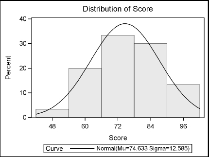
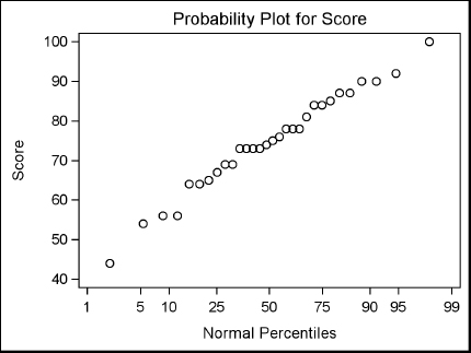
Example This example uses the data from the previous section, which consist of test scores from 30 students in a statistics class. The following program creates a histogram of the Score variable with the normal distribution overlaid, and a probability plot using the normal distribution:
LIBNAME f2020 'c:MySASLib';
*Create histogram and probability plot for variable Score;
PROC UNIVARIATE DATA = f2020.statclass;
VAR Score;
HISTOGRAM Score / NORMAL;
PROBPLOT Score;
TITLE;
RUN;
Here are the two plots: a histogram and a probability plot. (The NORMAL option in the HISTOGRAM statement produces additional tabular results that are not shown.) The relatively linear pattern formed by the points in the probability plot indicate that the data are closely matched to the normal distribution.
9.3 Producing Statistics with PROC MEANS
Most of the descriptive statistics that you produce with PROC UNIVARIATE you can also produce with PROC MEANS. PROC UNIVARIATE is useful when you want an in-depth statistical analysis of the data distribution. But if you know you want only a few statistics, then PROC MEANS is a better way to go. With PROC MEANS you can ask for just the statistics you want. The MEANS procedure does not produce any ODS Graphics.
The MEANS procedure requires only one statement:
PROC MEANS statistic-keywords;
If you do not include any statistic keywords, then MEANS will produce the mean, the number of nonmissing values, the standard deviation, the minimum value, and the maximum value for each numeric variable. The following table shows statistics you can request. (Some statistics have two names; the alternate name is shown in parentheses.) If you add any statistic keywords in the PROC MEANS statement, then MEANS will no longer produce the default statistics—you must request all the statistics you want.
|
CLM |
two-sided confidence limits |
RANGE |
range |
||
|
CSS |
corrected sum of squares |
SKEWNESS |
skewness |
||
|
CV |
coefficient of variation |
STDDEV |
standard deviation |
||
|
KURTOSIS |
kurtosis |
STDERR |
standard error of the mean |
||
|
LCLM |
lower confidence limit |
SUM |
sum |
||
|
MAX |
maximum value |
SUMWGT |
sum of weighted variables |
||
|
MEAN |
mean |
UCLM |
upper confidence limit |
||
|
MIN |
minimum value |
USS |
uncorrected sum of squares variance |
||
|
MODE |
mode |
VAR |
variance |
||
|
N |
number of nonmissing values |
PROBT |
probability for Student’s t |
||
|
NMISS |
number of missing values |
T |
Student’s t |
||
|
MEDIAN(P50) |
median |
Q3(P75) |
75% quantile |
||
|
Q1(P25) |
25% quantile |
P5 |
5% quantile |
||
|
P1 |
1% quantile |
P90 |
90% quantile |
||
|
P10 |
10% quantile |
P99 |
99% quantile |
||
|
P95 |
95% quantile |
|
|
|
|
Confidence limits The default confidence level for the confidence limits is .05 or 95%. If you want a different confidence level, then request it with the ALPHA= option in the PROC MEANS statement. For example, if you want 90% confidence limits, then specify ALPHA=.10 along with the CLM option. Then the PROC MEANS statement would look like this:
PROC MEANS ALPHA = .10 CLM;
VAR statement By default, PROC MEANS will produce statistics for all numeric variables in your data set. If you do not want all the variables, then specify the ones you want in the VAR statement. Here is the general form of the MEANS procedure with the VAR statement:
PROC MEANS options;
VAR variable-list;
Example Your friend is an aspiring author of children’s books. To increase her chances of getting her books published, she wants to know how many pages her books should have. At the local library, she counts the number of pages in a random selection of children’s picture books. Here are the data:
34 30 29 32 52 25 24 27 31 29
24 26 30 30 30 29 21 30 25 28
28 28 29 38 28 29 24 24 29 31
30 27 45 30 22 16 29 14 16 29
32 20 20 15 28 28 29 31 29 36
To determine the average number of pages in children’s picture books, use the MEANS procedure. PROC MEANS can also produce the median number of pages, as well as the 90% confidence limits. Here is the program that will read the data and produce the desired statistics:
DATA booklengths;
INFILE 'c:MyRawDataPicbooks.dat';
INPUT NumberOfPages @@;
RUN;
*Produce summary statistics;
PROC MEANS DATA = booklengths N MEAN MEDIAN CLM ALPHA = .10;
TITLE 'Summary of Picture Book Lengths';
RUN;
Here are the results of the MEANS procedure:
Summary of Picture Book Lengths
The MEANS Procedure
|
Analysis Variable : NumberOfPages |
||||
|
N |
Mean |
Median |
Lower 90% |
Upper 90% |
|
50 |
28.0000000 |
29.0000000 |
26.4419136 |
29.5580864 |
The average number of pages in the children’s books sampled was 28. The median value of 29 says that half the books sampled had 29 pages or fewer. The confidence limits tell us that we are 90% certain that the true population mean (all children’s picture books) falls between 26.44 and 29.56 pages. From this analysis your friend concludes that she should make her books between 26 and 30 pages long to maximize her chances of getting published (of course subject matter and writing style might also help).
9.4 Testing Means with PROC TTEST
As you would expect from its name, the TTEST procedure, which is part of SAS/STAT software, computes t tests. You use t tests when you want to compare means. Suppose, for example, that a statistics instructor selected a random sample of students to have extra tutoring. She could test whether the true mean of their scores was above a specific level (called a one-sample test), she could compare the scores of students who had tutoring to those who did not (a two independent sample test), and she could compare the scores of students before and after tutoring (a paired test). PROC TTEST performs all these types of tests.
One sample comparisons To compute a t test for a single mean, you list that variable in a VAR statement. SAS will test whether the mean is significantly different from H0, a specified null value. The default value of H0 is zero. You can specify a different value using the H0= option.
PROC TTEST H0 = n options;
VAR variable;
Two independent sample comparisons To compare two independent groups, you use a CLASS and a VAR statement. In the CLASS statement, you list the variable that distinguishes the two groups. In the VAR statement, you list the response variable.
PROC TTEST options;
CLASS variable;
VAR variable;
Paired comparisons When the variables that you are comparing are paired, you use a PAIRED statement. The simplest form of this statement lists the two variables to be compared, separated by an asterisk.
PROC TTEST options;
PAIRED variable1 * variable2;
Options Here are a few of the options available:
ALPHA = n specifies the level for the confidence limits. The value of n must be between 0 (100% confidence) and 1 (0% confidence). The default is 0.05 (95% confidence limits).
CI = type specifies the type of confidence interval for the standard deviation. If you don't specify this option, then by default the value of type is EQUAL, which produces an equal-tailed confidence interval. Other possible values are UMPU for an interval based on the uniformly most powerful unbiased test, and NONE to request no confidence interval for the standard deviation.
H0 = n requests a test of the hypothesis H0 = n. The default value is 0.
NOBYVAR moves the names of the variables from the title to the output table.
SIDES = type specifies whether the p-value and confidence interval are one or two-tailed. Possible values of type are 2 (the default) for two-tailed, L (for a lower one-sided test) or U (for an upper one-sided test).
Example The following data give the finishing times for semifinal and final races of the women’s 50-meter freestyle swim. Each swimmer’s initials are followed by their final time and semifinal time in seconds. Each line of data contains times for four swimmers.
RK 24.05 24.07 AH 24.28 24.45 MV 24.39 24.50 BS 24.46 24.57
FH 24.47 24.63 TA 24.61 24.71 JH 24.62 24.68 AV 24.69 24.64
The following program reads the raw data and uses a paired t test to test the mean difference between the semifinal and final times:
LIBNAME results 'c:MySASLib';
DATA results.swim;
INFILE 'c:MyRawDataOlympic50mSwim.dat';
INPUT Swimmer $ FinalTime SemiFinalTime @@;
RUN;
*Perform paired t test for semifinal and final times;
PROC TTEST DATA = results.swim;
TITLE '50m Freestyle Semifinal vs. Final Results';
PAIRED SemiFinalTime * FinalTime;
RUN;
Here are the tabular results produced by PROC TTEST. Graphical results are shown in the next section.
50m Freestyle Semifinal vs. Final Results
|
The TTEST Procedure |
|
Difference: SemiFinalTime - FinalTime |
|
N |
Mean |
Std Dev |
Std Err |
Minimum |
Maximum |
|
8 |
0.0850 |
0.0731 |
0.0258 |
-0.0500 |
0.1700 |
|
Mean |
95% CL Mean |
Std Dev |
95% CL Std Dev |
||
|
0.0850 |
0.0239 |
0.1461 |
0.0731 |
0.0483 |
0.1488 |
|
DF |
t Value |
Pr > |t| |
|
7 |
3.29 |
0.0133 |
In this example, the mean difference between each swimmer’s semifinal time and their final time is 0.0850 seconds. The t test shows significant evidence (DF=7, t= 3.29, p = 0.0133) of a difference between the mean semifinal and final times.
9.5 Creating Statistical Graphics with PROC TTEST
The TTEST procedure uses ODS Graphics to produce several plots that help you visualize your data including histograms, box plots, and Q-Q plots. Many plots are generated by default, but you can control which plots are created using the PLOTS option in the PROC TTEST statement. Here is the general form of the PROC TTEST statement with plot options:
PROC TTEST PLOTS = (plot-request-list);
Plot requests The plots available to you depend on the type of comparison you request. Here are plots you can request for one sample, two sample, and paired t tests:
ALL all appropriate plots
BOXPLOT box plots
HISTOGRAM histograms overlaid with normal and kernel density curves
INTERVALPLOT plots of confidence interval of means
NONE no plots
QQPLOT normal quantile-quantile (Q-Q) plot
SUMMARYPLOT one plot that includes both histograms and box plots
The following plots are also available for paired t tests:
AGREEMENTPLOT agreement plots
PROFILESPLOT profiles plot
Excluding automatic plots By default the QQPLOT and SUMMARYPLOT plots are generated automatically for one sample, two sample and paired t tests. For paired t tests, the AGREEMENTPLOT and PROFILESPLOT are also generated by default. If you choose specific plots in the plot-list, the default plots will still be created unless you add the ONLY global option:
PROC TTEST PLOTS(ONLY) = (plot-request-list);
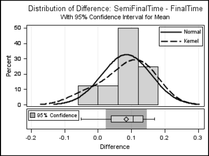
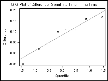
Example This example uses the data from the previous section, which gives the finishing times for semifinal (SemiFinalTime) and final races (FinalTime) of the women’s 50-meter freestyle swim. The following program uses a paired t test to test the mean difference between the semifinal and final times, and requests just the Summary and Q-Q plots.
LIBNAME results 'c:MySASLib';
*Produce just the Summary and QQ plots;
PROC TTEST DATA = results.swim PLOTS(ONLY) = (SUMMARYPLOT QQPLOT);
TITLE '50m Freestyle Semifinal vs. Final Results';
PAIRED SemiFinalTime * FinalTime;
RUN;
Here are the results for the Q-Q and Summary plots. The tabular results for the paired t test were shown in the preceding section.
9.6 Testing Categorical Data with PROC FREQ
PROC FREQ, which is part of Base SAS, produces many statistics for categorical data. The best known of these is chi-square. One of the most common uses of PROC FREQ is to test the hypothesis of no association between two variables. Another use is to compute measures of association, which indicate the strength of the relationship between the variables. The general form of PROC FREQ is:
PROC FREQ;
TABLES variable-combinations / options;
Options Here are a few of the statistical options that you can request:
|
AGREE |
tests and measures of classification agreement, including McNemar’s test, Bowker’s test, Cochran’s Q test, and kappa statistics |
|
CHISQ |
chi-square tests of independence and measures of association |
|
CL |
confidence limits for measures of association |
|
CMH |
Cochran-Mantel-Haenszel statistics, typically for stratified two-way tables |
|
EXACT |
Fisher’s exact test for tables larger than 2X2 |
|
MEASURES |
measures of association, including Pearson and Spearman correlation coefficients, gamma, Kendall’s tau-b, Stuart’s tau-c, Somer’s D, lambda, odds ratios, risk ratios, and confidence intervals |
|
RELRISK |
relative risk measures for 2X2 tables |
|
TREND |
Cochran-Armitage test for trend |
Example One day your neighbor, who rides the bus to work, complains that the regular bus is usually late. He says the express bus is usually on time. Realizing that this is categorical data, you decide to test whether there really is a relationship between the type of bus and arriving on time. You collect data for type of bus (E for express or R for regular) and promptness (L for late or O for on time). Each line of data contains several observations.
E O E L E L R O E O E O E O R L R O R L R O E O R L E O R L R O E O
E O R L E L E O R L E O R L E O R L E O R O E L E O E O E O E O E L
E O E O R L R L R O R L E L E O R L R O E O E O E O E L R O R L
The following program reads the raw data and runs PROC FREQ with the CHISQ option:
LIBNAME trans 'c:MySASLib';
DATA trans.bus;
INFILE 'c:MyRawDataBus.dat';
INPUT BusType $ OnTimeOrLate $ @@;
RUN;
*Perform chi-square analysis on bus data;
PROC FREQ DATA = trans.bus;
TABLES BusType * OnTimeOrLate / CHISQ;
TITLE;
RUN;
Here are the results showing that the regular bus is late 61.90% of the time, while the express bus is late only 24.14% of the time. Assuming that bus type and arrival time are independent, the probability of obtaining a chi-square this large or larger by chance alone is 0.0071. So the data do support the idea that there is an association between type of bus and arrival time. The Fisher’s exact test provides the same conclusion with a p-value of 0.0097.
The FREQ Procedure
|
Table of BusType by OnTimeOrLate |
|||
|
BusType |
OnTimeOrLate |
||
|
Frequency |
L |
O |
Total |
|
E |
7 |
22 |
29 |
|
R |
13 |
8 |
21 |
|
Total |
20 |
30 |
50 |
Statistics for Table of BusType by OnTimeOrLate
|
Statistic |
DF |
Value |
Prob |
|
|
Chi-Square |
1 |
7.2386 |
0.0071 |
|
|
Likelihood Ratio Chi-Square |
1 |
7.3364 |
0.0068 |
|
|
Continuity Adj. Chi-Square |
1 |
5.7505 |
0.0165 |
|
|
Mantel-Haenszel Chi-Square |
1 |
7.0939 |
0.0077 |
|
|
Phi Coefficient |
|
-0.3805 |
|
|
|
Contingency Coefficient |
|
0.3556 |
|
|
|
Cramer's V |
|
-0.3805 |
|
|
|
Fisher's Exact Test |
|
|
Cell (1,1) Frequency (F) |
7 |
|
Left-sided Pr <= F |
0.0081 |
|
Right-sided Pr >= F |
0.9987 |
|
|
|
|
Table Probability (P) |
0.0067 |
|
Two-sided Pr <= P |
0.0097 |
|
Sample Size = 50 |
9.7 Creating Statistical Graphics with PROC FREQ
The FREQ procedure uses ODS Graphics to produce several plots that help you visualize your data including frequency plots, odds ratio plots, agreement plots, deviation plots, and two types of plots with Kappa statistics and confidence limits. Here is the general form of PROC FREQ with plot options:
PROC FREQ;
TABLES variable-combinations / options PLOTS = (plot-list);
Plot requests The plots available to you depend on the type of table you request. For example, the DEVIATIONPLOT is available only for one-way tables when using the CHISQ option in the TABLES statement. Here are the plots that you can request along with the required option, if any, and type of table request:
|
Plot Name |
Table type |
Required option in TABLES statement |
|
AGREEPLOT |
two-way |
AGREE |
|
CUMFREQPLOT |
one-way |
|
|
DEVIATIONPLOT |
one-way |
CHISQ |
|
FREQPLOT |
any request |
|
|
KAPPAPLOT |
three-way |
AGREE |
|
ODDSRATIOPLOT |
hx2x2 |
MEASURES or RELRISK |
|
RELREISKPLOT |
hx2x2 |
MEASURES or RELRISK |
|
RISKDIFFPLOT |
hx2x2 |
RISKDIFF |
|
WTKAPPAPLOT |
hxrxr (r>2) |
AGREE |
To produce a CUMFREQPLOT or a FREQPLOT, you must specify it in the PLOTS= option in the TABLES statement. Otherwise, if you do not specify any plots in the TABLE statement, then all plots associated with the table type you request will be produced by default.
Plot options Many options are available that control the look of the plots generated. For a complete list of options, see the SAS Documentation. For example, the FREQPLOT has options for controlling the layout of the plots for two-way tables. By default, the bars are grouped vertically. To group the bars horizontally, use the following:
TABLES variable1 * variable2 / PLOTS = FREQPLOT(TWOWAY = GROUPHORIZONTAL);
To stack the bars, use the TWOWAY=STACKED option.
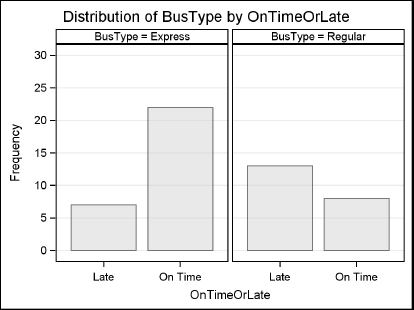
Example This example uses the same data as the previous section about promptness of buses. The data are for type of bus (E for express or R for regular) and promptness (L for late or O for on time). The following program uses PROC FREQ to request a two-way frequency table. The PLOTS=FREQPLOT option in the TABLES statement produces a frequency plot. Adding the TWOWAY=GROUPHORIZONTAL option to FREQPLOT produces bars that are grouped horizontally instead of vertically. The FORMAT procedure creates formats that are applied to the BusType and OnTimeOrLate variables using a FORMAT statement in the FREQ procedure. This gives more descriptive labels to the plot.
LIBNAME trans 'c:MySASLib';
PROC FORMAT;
VALUE $type 'R'='Regular'
'E'='Express';
VALUE $late 'O'='On Time'
'L'='Late';
RUN;
*Produce frequency plot grouped horizontally;
PROC FREQ DATA = trans.bus;
TABLES BusType * OnTimeOrLate / PLOTS=FREQPLOT(TWOWAY=GROUPHORIZONTAL);
FORMAT BusType $Type. OnTimeOrLate $Late.;
RUN;
Here is the plot. The tabular portion of the output, the frequency table, was shown in the previous section.
9.8 Examining Correlations with PROC CORR
The CORR procedure, which is included with Base SAS, computes correlations. A correlation coefficient measures the strength of the linear relationship between two variables. If two variables are completely unrelated, they will have a correlation of 0. If two variables have a perfect linear relationship, they will have a correlation of 1.0 or –1.0. In real life, correlations fall somewhere between these numbers. The basic syntax for PROC CORR is rather simple:
PROC CORR;
RUN;
By default, SAS will compute correlations between all possible pairs of the numeric variables. You can add the VAR and WITH statements to specify variables:
VAR variable-list;
WITH variable-list;
Variables listed in the VAR statement appear across the top of the table of correlations, while variables listed in the WITH statement appear down the side of the table. If you use a VAR statement but no WITH statement, then the variables will appear both across the top and down the side.
By default, PROC CORR computes Pearson product-moment correlation coefficients. You can add options to the PROC statement to request nonparametric correlation coefficients. The SPEARMAN option in the statement below tells SAS to compute Spearman’s rank correlations instead of Pearson’s correlations:
PROC CORR SPEARMAN;
Other options include HOEFFDING (for Hoeffding’s D statistic) and KENDALL (for Kendall’s tau-b coefficient).
Example Each student in a statistics class recorded three values: test score, the number of hours spent watching videos in the week prior to the test, and the number of hours spent exercising during the same week. Here are the raw data:
56 6 2 78 7 4 84 5 5 73 4 0 90 3 4
44 9 0 76 5 1 87 3 3 92 2 7 75 8 3
85 1 6 67 4 2 90 5 5 84 6 5 74 5 2
64 4 1 73 0 5 78 5 2 69 6 1 56 7 1
87 8 4 73 8 3 100 0 6 54 8 0 81 5 4
78 5 2 69 4 1 64 7 1 73 7 3 65 6 2
Notice that each line contains data for five students. The following program reads the raw data from a file called Exercise.dat, and then uses PROC CORR to compute the correlations:
LIBNAME mylib 'c:MySASLib';
DATA mylib.class;
INFILE 'c:MyRawDataExercise.dat';
INPUT Score Videos Exercise @@;
RUN;
*Perform correlation analysis;
PROC CORR DATA = mylib.class;
VAR Videos Exercise;
WITH Score;
TITLE 'Correlations for Test Scores';
TITLE2 'With Hours of Videos and Exercise';
RUN;
Here is the report from PROC CORR:
Correlations for Test Scores
With Hours of Videos and Exercise
|
The CORR Procedure |
|
1 With Variables: |
Score |
|
2 Variables: |
Videos Exercise |
|
Simple Statistics |
||||||
|
Variable |
N |
Mean |
Std Dev |
Sum |
Minimum |
Maximum |
|
Score |
30 |
74.63333 |
12.58484 |
2239 |
44.00000 |
100.00000 |
|
Videos |
30 |
5.10000 |
2.33932 |
153.00000 |
0 |
9.00000 |
|
Exercise |
30 |
2.83333 |
1.94906 |
85.00000 |
0 |
7.00000 |
❶ Pearson Correlation Coefficients, N = 30 ❷ Prob > |r| under H0: Rho=0 |
||
|
|
Videos |
Exercise |
|
Score |
❶ -0.55390 |
❶ 0.79733 |
This report starts with descriptive statistics for each variable, and then lists the correlation matrix, which contains: ❶correlation coefficients (in this case, Pearson), and ❷ the probability of getting a larger absolute value for each correlation assuming that the population correlation is zero.
In this example, both hours of videos and hours of exercise are correlated with test score, but exercise is positively correlated while videos is negatively correlated. This means students who watched more videos tended to have lower scores, while the students who spent more time exercising tended to have higher scores.
9.9 Creating Statistical Graphics with PROC CORR
The CORR procedure evaluates the strength of the linear relationship between pairs of variables. The tabular output gives the correlation coefficients and other simple statistics, and using ODS Graphics you can also visualize the relationship. Plots are not generated by default, so you need to specify the desired plots using the PLOTS= option. Here is the general form of PROC CORR with the PLOTS option:
PROC CORR PLOTS = (plot-list);
VAR variable-list;
WITH variable-list;
Plot requests The CORR procedure can create two types of plots:
|
SCATTER |
scatter plots for pairs of variables overlaid with prediction or confidence ellipses |
|
MATRIX |
matrix of scatter plots for all variables |
Plot options By default, the scatter plots include prediction ellipses for new observations. If you want confidence ellipses for means, then specify the ELLIPSE=CONFIDENCE option on the scatter plot:
PROC CORR PLOTS = SCATTER(ELLIPSE = CONFIDENCE);
If you do not want any ellipses on your scatter plots, then use the ELLIPSE=NONE option.
If you do not have a WITH statement, then matrix plots will show a symmetrical plot with all variable combinations appearing twice. By default the diagonal cells in the matrix will be empty. If you use the HISTOGRAM option for the matrix plot, then a histogram will be produced for each variable and displayed along the diagonal.
PROC CORR PLOTS = MATRIX(HISTOGRAM);
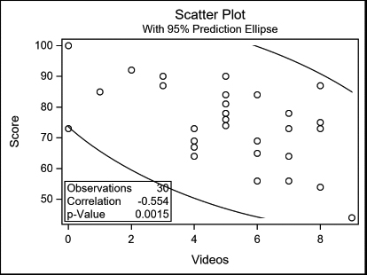
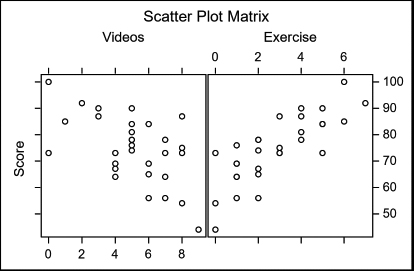
Example This example uses the data from the previous section about students in a statistics class. For each student, we have the test score (Score), the number of hours spent watching videos in the week prior to the test (Videos), and the number of hours spent exercising during the same week (Exercise). The following program uses the same PROC CORR statements shown in the previous section except both the scatter and matrix plots are requested:
LIBNAME mylib 'c:MySASLib';
*Generate scatter and matrix plots for correlation analysis;
PROC CORR DATA = mylib.class PLOTS = (SCATTER MATRIX);
VAR Videos Exercise;
WITH Score;
TITLE 'Correlations for Test Scores';
TITLE2 'With Hours of Videos and Exercise';
RUN;
The program produces three plots: a scatter plot for Score by Videos, a scatter plot for Score by Exercise (not shown), and the Scatter Plot Matrix.
9.10 Using PROC REG for Simple Regression Analysis
The REG procedure fits linear regression models by least squares and is one of many SAS procedures that perform regression analysis. PROC REG is part of SAS/STAT, which is licensed separately from Base SAS. We will show an example of a simple regression analysis using continuous numeric variables with only one regressor variable. However, PROC REG is capable of analyzing models with many regressor variables using a variety of model-selection methods, including stepwise regression, forward selection, and backward elimination. Other procedures in SAS/STAT will perform non-linear and logistic regression. In SAS/ETS, you will find procedures for time series analysis. If you are unsure about what type of analysis you need, or are unfamiliar with basic statistical principles, we recommend that you seek advice from a trained statistician, or consult a good statistical textbook.
The REG procedure has only two required statements. It must start with the PROC REG statement and have a MODEL statement specifying the analysis model. Here is the general form:
PROC REG;
MODEL dependent = independent;
In the MODEL statement, the dependent variable is listed on the left side of the equal sign and the independent, or regressor, variable is listed on the right.
Example At your young neighbor’s T-ball game (that’s where the players hit the ball from the top of a tee instead of having the ball pitched to them), he said to you, “You can tell how far they’ll hit the ball by how tall they are.” To give him a little practical lesson in statistics, you decide to test his hypothesis. You gather data from 30 players, measuring their height in inches and their longest of three hits in feet. The following are the data. Notice that data for several players are listed on one line:
50 110 49 135 48 129 53 150 48 124 50 143 51 126 45 107
53 146 50 154 47 136 52 144 47 124 50 133 50 128 50 118
48 135 47 129 45 126 48 118 45 121 53 142 46 122 47 119
51 134 49 130 46 132 51 144 50 132 50 131
The following program reads the data and performs the regression analysis. In the MODEL statement, Distance is the dependent variable, and Height is the independent variable.
LIBNAME tball 'c:MySASLib';
DATA tball.hits;
INFILE 'c:MyRawDataBaseball.dat';
INPUT Height Distance @@;
RUN;
* Perform regression analysis;
PROC REG DATA = tball.hits;
MODEL Distance = Height;
TITLE 'Results of Regression Analysis';
RUN;
The REG procedure produces tabular results and several graphs by default. Only the tabular results are shown here; see the next section for an example showing the graphical results. The first section of the tabular output is the analysis of variance section, which gives information about how well the model fits the data:
Results of Regression Analysis
|
The REG Procedure |
|||
|
Number of Observations Read |
30 |
|
|
Number of Observations Used |
30 |
|
|
Analysis of Variance |
|||||
|
Source |
❶ DF |
Sum of Squares |
❷ Mean Square |
❸ F Value |
❹ Pr > F |
|
Model |
1 |
1365.50831 |
1365.50831 |
16.86 |
0.0003 |
|
Error |
28 |
2268.35836 |
81.01280 |
|
|
|
Corrected Total |
29 |
3633.86667 |
|
|
|
|
❺ Root MSE |
9.00071 |
R-Square |
0.3758 |
|
Dependent Mean |
130.73333 |
❼ Adj R-Sq |
0.3535 |
|
❻ Coeff Var |
6.88479 |
|
|
|
❶ DF |
degrees of freedom associated with the source |
|
❷ Mean Square |
mean square (sum of squares divided by the degrees of freedom) |
|
❸ F value |
F value for testing the null hypothesis (all parameters are zero except intercept) |
|
❹ Pr > F |
significance probability or p-value |
|
❺ Root MSE |
root mean square error |
|
❻ Coeff Var |
the coefficient of variation |
|
❼ Adj R-sq |
the R-square value adjusted for degrees of freedom |
The parameter estimates follow the analysis of variance section and give the parameters for each term in the model, including the intercept:
|
Parameter Estimates |
|||||
|
Variable |
❶ DF |
Parameter Estimate |
Standard Error |
❷ t Value |
❸ Pr > |t| |
|
Intercept |
1 |
-11.00859 |
34.56363 |
-0.32 |
0.7525 |
|
Height |
1 |
2.89466 |
0.70506 |
4.11 |
0.0003 |
|
❶ DF |
degrees of freedom for the variable |
|
❷ t Value |
t test for the parameter equal to zero |
|
❸ Pr > |t| |
two-tailed significance probability |
From the parameter estimates you can construct the regression equation:
Distance = -11.00859 + (2.89466 * Height)
In this example, the distance the ball was hit did increase with the player’s height. The slope of the model is significant (p= 0.0003) but the relationship is not very strong (R-square = 0.3758). Perhaps age or years of experience are better predictors of how far the ball will go.
9.11 Creating Statistical Graphics with PROC REG
There are many plots that are useful for visualizing the results of regression analysis and for assessing how well the model fits the data. PROC REG uses ODS Graphics to produce many such plots, including a diagnostic panel that contains up to nine plots in one figure. Some plots are produced automatically while others need to be specified. Here is the general form of PROC REG with the PLOTS option:
PROC REG PLOTS(options) = (plot-request-list);
MODEL dependent = independent;
Plot requests Here are some plots that you can request for simple linear regression:
|
FITPLOT |
scatter plot with regression line and confidence and prediction bands |
|
RESIDUALS |
residuals plotted against independent variable |
|
DIAGNOSTICS |
diagnostics panel including all of the following plots |
|
COOKSD |
Cook’s D statistic by observation number |
|
OBSERVEDBYPREDICTED |
dependent variable by predicted values |
|
QQPLOT |
normal quantile plot of residuals |
|
RESIDUALBYPREDICTED |
residuals by predicted values |
|
RESIDUALHISTOGRAM |
histogram of residuals |
|
RFPLOT |
residual fit plot |
|
RSTUDENTBYLEVERAGE |
studentized residuals by leverage |
|
RSTUDENTBYPREDICTED |
studentized residuals by predicted values |
Excluding automatic plots By default, the RESIDUALS and DIAGNOSTICS plots are generated automatically. Additional plots may also be produced by default depending on the type of model. For example, a FITPLOT is automatically generated when there is one regressor variable. If you choose specific plots in the plot-request-list, the default plots will still be created unless you use the ONLY global option:
PROC REG PLOTS(ONLY) = (plot-request-list);
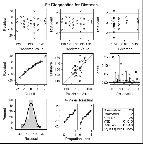
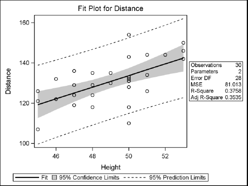
Example The following example uses the same data as the previous section about T-ball players. The data are the player’s height in inches (Height) and their longest of three hits in feet (Distance). The following program performs the regression analysis as in the previous section. However, in this program only the FITPLOT and DIAGNOSTICS plots are requested:
LIBNAME tball 'c:MySASLib';
*Limit plots generated to diagnostics panel and fit plot;
PROC REG DATA = tball.hits PLOTS(ONLY) = (DIAGNOSTICS FITPLOT);
MODEL Distance = Height;
TITLE 'Results of Regression Analysis';
RUN;
Here are the results for the Fit Diagnostics panel and the Fit Plot. The tabular results are not shown here, but are the same as in the previous section.
9.12 Using PROC ANOVA for One-Way Analysis of Variance
The ANOVA procedure is one of many in SAS that perform analysis of variance. PROC ANOVA is part of SAS/STAT, which is licensed separately from Base SAS. PROC ANOVA is specifically designed for balanced data—data where there are equal numbers of observations in each combination of the classification factors. An exception is for one-way analysis of variance where the data do not need to be balanced. If you are not doing one-way analysis of variance and your data are not balanced, then you should use the GLM procedure, whose statements are almost identical to those of PROC ANOVA. Although we are discussing only simple one-way analysis of variance in this section, PROC ANOVA can handle multiple classification variables and models that include nested and crossed effects as well as repeated measures. If you are unsure of the appropriate analysis for your data, or are unfamiliar with basic statistical principles, we recommend that you seek advice from a trained statistician or consult a good statistical textbook.
The ANOVA procedure has two required statements: the CLASS and MODEL statements. Here is the general form of the ANOVA procedure:
PROC ANOVA;
CLASS variable-list;
MODEL dependent = effects;
The CLASS statement must come before the MODEL statement and defines the classification variables. For one-way analysis of variance, only one variable is listed. The MODEL statement defines the dependent variable and the effects. For one-way analysis of variance, the effect is the classification variable.
As you might expect, there are many optional statements for PROC ANOVA. One of the most useful is the MEANS statement, which calculates means of the dependent variable for any of the main effects in the MODEL statement. In addition, the MEANS statement can perform several types of multiple-comparison tests, including Bonferroni t tests (BON), Duncan’s multiple-range test (DUNCAN), Scheffe’s multiple-comparison procedure (SCHEFFE), pairwise t tests (T), and Tukey’s studentized range test (TUKEY). The MEANS statement has the following general form:
MEANS effects / options;
The effects can be any effect in the MODEL statement, and options include the name of the desired multiple-comparison test (DUNCAN for example).
Example Your friend’s daughter plays basketball on a team that travels throughout the state. She complains that it seems like the girls from the other regions in the state are all taller than the girls from her region. You decide to test her hypothesis by getting the heights for a sample of girls from the four regions and performing one-way analysis of variance to see if there are any differences. Each data line includes region and height for eight girls:
West 65 West 58 West 63 West 57 West 61 West 53 West 56 West 66
West 55 West 56 West 65 West 54 West 55 West 62 West 55 West 58
East 65 East 55 East 57 East 66 East 59 East 63 East 58 East 57
East 58 East 63 East 61 East 62 East 58 East 57 East 65 East 57
South 63 South 63 South 68 South 56 South 60 South 65 South 64 South 62
South 59 South 67 South 59 South 65 South 66 South 67 South 64 South 68
North 63 North 65 North 58 North 55 North 57 North 66 North 59 North 61
North 65 North 56 North 57 North 63 North 61 North 60 North 64 North 62
You want to know which, if any, regions have taller girls than the rest, so you use the MEANS statement in your program and choose Scheffe’s multiple-comparison method to compare the means. Here is the program to read the data and perform the analysis of variance:
DATA heights;
INFILE 'c:MyRawDataGirlHeights.dat';
INPUT Region $ Height @@;
RUN;
* Use ANOVA to run one-way analysis of variance;
PROC ANOVA DATA = heights;
CLASS Region;
MODEL Height = Region;
MEANS Region / SCHEFFE;
TITLE "Girls' Heights from Four Regions";
RUN;
In this case, Region is the classification variable and also the effect in the MODEL statement. Height is the dependent variable. The MEANS statement will produce means of the girls’ heights for each region, and the SCHEFFE option will test which regions are different from the others.
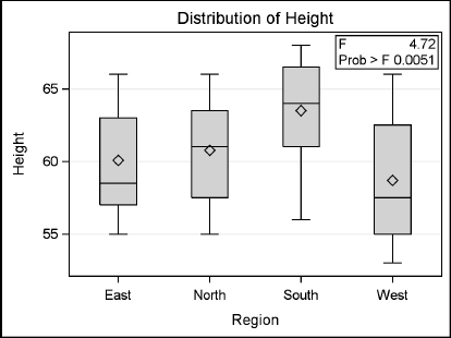
Here is the box plot that is created automatically. The small p-value (p=0.0051) indicates that at least two of the four regions differ in mean height. The tabular output is shown and discussed in the next section.
9.13 Reading the Output of PROC ANOVA
The tabular output from PROC ANOVA has at least two parts. First, ANOVA produces a table giving information about the classification variables: number of levels, values, and number of observations. Next, it produces an analysis of variance table. If you use optional statements like MEANS, then their output will follow.
The example from the previous section used the following PROC ANOVA statements:
PROC ANOVA DATA = heights;
CLASS Region;
MODEL Height = Region;
MEANS Region / SCHEFFE;
TITLE "Girls' Heights from Four Regions";
RUN;
The graph produced by the ANOVA procedure is shown in the previous section. The first page of the tabular output (shown below) gives information about the classification variable Region. It has four levels with values East, North, South, and West; and there are 64 observations.
Girls' Heights from Four Regions
|
The ANOVA Procedure |
|
Class Level Information |
||
|
Class |
Levels |
Values |
|
Region |
4 |
East North South West |
|
Number of Observations Read |
64 |
|
Number of Observations Used |
64 |
The second part of the output is the analysis of variance table:
Girls' Heights from Four Regions
|
The ANOVA Procedure |
|
Dependent Variable: Height |
|
❶ Source |
❷ DF |
❸ Sum of Squares |
❹ Mean Square |
❺ F Value |
❻ Pr > F |
|
Model |
3 |
196.625000 |
65.541667 |
4.72 |
0.0051 |
|
Error |
60 |
833.375000 |
13.889583 |
|
|
|
Corrected Total |
63 |
1030.000000 |
|
|
|
|
❼ R-Square |
❽ Coeff Var |
❾ Root MSE |
❿ Height Mean |
|
0.190898 |
6.134771 |
3.726873 |
60.75000 |
|
Source |
DF |
Anova SS |
Mean Square |
F Value |
Pr > F |
|
Region |
3 |
196.6250000 |
65.5416667 |
4.72 |
0.0051 |
Highlights of the output are:
|
❶ Source |
source of variation |
|
❷ DF |
degrees of freedom for the model, error, and total |
|
❸ Sum of Squares |
sum of squares for the portion attributed to the model, error, and total |
|
❹ Mean Square |
mean square (sum of squares divided by the degrees of freedom) |
|
❺ F Value |
F value (mean square for model divided by the mean square for error) |
|
❻ Pr > F |
significance probability associated with the F statistic |
|
❼ R-Square |
R-square |
|
❽ Coeff Var |
coefficient of variation |
|
❾ Root MSE |
root mean square error |
|
❿ Height Mean |
mean of the dependent variable |
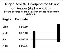
Because the effect of Region is significant (p = .0051), we conclude that there are differences in the mean heights of girls from the four regions. The SCHEFFE option in the MEANS statement compares the mean heights between the regions. The following results show that your friend’s daughter is partially correct—one region (South) has taller girls than her region (West) but no other two regions differ significantly in mean height. Older versions of SAS may display a table instead of a graph. If you prefer a table, then add the LINESTABLE option to the MEANS statement.
Girls' Heights from Four Regions
|
The ANOVA Procedure |
|
Scheffe's Test for Height |
Note: This test controls the Type I experimentwise error rate.
|
Alpha |
0.05 |
|
Error Degrees of Freedom |
60 |
|
Error Mean Square |
13.88958 |
|
Critical Value of F |
2.75808 |
|
Minimum Significant Difference |
3.7902 |