Key words

permeability; diffusion; computer model; finite difference; finite step

2.1 Introduction

Having defined the basic physical equations in Chapter 1, there are two possible ways to make use of them: they may be integrated either analytically or numerically. Both approaches are used in different chapters of this book. In this chapter, a simple approach to numerical integration using BASIC computer code is described. This numerical integration may also be described as finite step modelling. The computer modelling was carried out using code written in Visual Basic running as a macro in Microsoft Excel on a standard desktop computer.

There are many different software packages available which can be used for modelling of this type. However, the author is not aware of any that can model the particular complexities that arise in the transport processes in concrete. In particular for the electromigration model, which is used in several of the later chapters of this book, there do not appear to be any packages that can adequately account for charge conservation. Also when considering pressure-driven flow combined with diffusion in a multilayer containment barrier, no packages were found that could be used for modelling. It must also be observed that a simple model for, say, pressure-driven flow combined with diffusion can be written in a few hours and will run on any computer with Microsoft Excel without the need to locate and purchase a package. The main limitation of this type of programme is that it is one-dimensional and can only model situations in which the flow is linear or there is, for example, circular, cylindrical or spherical symmetry.

To give an example of how the code can be written, combined pressure-driven flow and diffusion through a barrier is considered. The use of this particular model is described in Chapter 15 which also explains the purpose of the three layers. The same programme was used to analyse the three-layer barriers used in the site trials and the single-layer samples tested in the laboratory.

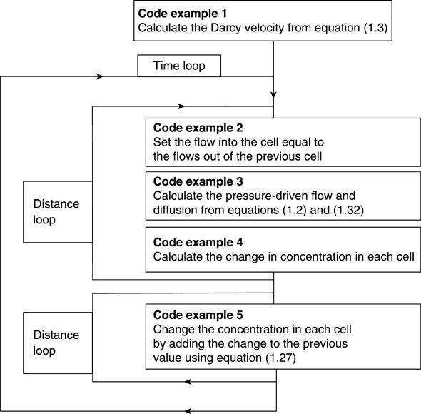
The structure of the programme is shown in Fig. 2.1; it loops through the sample in time and space. Examples of the code are discussed in Section 2.2.

2.2 Expressing the basic equations as computer code

2.2.2 Code example 1: calculation of Darcy velocity

The computer code is complicated by the fact that this code was written for a multi-layer barrier. The Darcy velocity is calculated as follows:

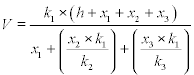$V=\frac{k_1\times \left(h+x_1+x_2+x_3\right)}{x_1+\left(\frac{x_2\times k_1}{k_2}\right)+\left(\frac{x_3\times k_1}{k_3}\right)}$ [2.1]

[2.1]

where h is the total height of the water column on the sample which is added to the height (thickness) of the sample itself if the flow through it is vertical, but not if it is horizontal (as in lab tests).

The variables are expressed in the computer code as follows:

k1	PERM (1)	element 1 in an array of permeabilities
H + x1 + x2 + x3	tHeight	the total height (thickness) of the barrier
x1	THICK (1)	the thickness of layer 1

Thus the code for equation (2.1) becomes:

V = PERM (1) * (tHeight) / (THICK (1) = (THICK (2) * PERM (l) / PERM (2)) + (THICK (3) * PERM (l) / PERM (3))) [Code example 1]

2.2.3 Code example 2: updating input to cell

The sample is divided up into cells as shown in Fig. 2.2, where cin and cout are the total flows due to pressure-driven flow during the time step and din and dout are the flows for diffusion. As the programme moves to consider the next cell, the flow out of the previous one becomes the flow into the next. The code for this is:

cin = cout

din = dout [Code example 2]

2.2.4 Code example 3: advection and diffusion calculation

Advection calculation

The advection from cell i to cell i + 1 during a single time step dt is calculated as:

$F\times \text{d}t=\text{d}t\times V\times C{l}_i$ [2.2]

[2.2]

The variable dt is expressed as dtd in the code so it becomes:

cout = V * dtd * CL (I) [Code example 3a]

where:

CL (I) = Cl_i, the concentration in the liquid in cell i

V is the Darcy velocity of the flow and

dtd is the time step.

Diffusion calculation

The cells may be in different layers of the barrier with different porosities, diffusion coefficients and cell thicknesses. The formula assumes that cell sizes have been set so all cells are entirely in a single layer and thus do not have a layer boundary in them.

The diffusion from cell i to cell i + 1 during a single time step dt is calculated as:

$F\text{d}t=\text{d}t\frac{C_{1_i}-C_{1_{\left(i+1\right)}}}{\left(\frac{C{t}_i}{\left(2D_i{\epsilon }_i\right)}+\frac{C{t}_{i+1}}{\left(2D_{i+1}{\epsilon }_{i+1}\right)}\right)}$ [2.3]

[2.3]

where Ct_i is the cell thickness.

For the code, clayer is the layer in which the current cell (I) is located and nlayer is the layer in which the next cell (I + 1) is located. IDIF (clayer), POR (clayer) and CTHICK (clayer) are the intrinsic diffusion coefficient, porosity and cell thickness for the layer in which the cell I is located. The code for equation (2.3) therefore becomes:

dout = dtd * (CL (I) = CL (I + l)) / ((CTHICK (clayer) / (2 * IDIF (clayer) * POR (clayer))) = (CTHICK (nlayer) / (2 * IDIF (nlayer) * POR (nlayer)))) [Code example 3b]

For the upper and lower cells (numbers 1 and n), the diffusion is doubled because the diffusion path to the centre of the cell only runs through half the distance of solid.

2.3 Other elements of the code

2.3.1 Checking the code

Transport by advection alone reaches a steady state when the concentration throughout the barrier $C_{{\text{s}}_i}$ = the concentration above it $C_{{\text{s}}_0}$. Thus:

$F=V\times C_{{\text{s}}_0}$ [2.4]

[2.4]

Transport by diffusion alone reaches a steady state when there is a linear concentration gradient through the barrier. The flux is given by:

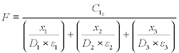$F=\frac{C_{1_0}}{\left(\frac{x_1}{D_1\times {\epsilon }_1}\right)+\left(\frac{x_2}{D_2\times {\epsilon }_2}\right)+\left(\frac{x_3}{D_3\times {\epsilon }_3}\right)}$ [2.5]

[2.5]

These values are calculated at the start of the programme and can be used for checking purposes.

The steady state values were checked by hand calculation and, for a number of different configurations, the programme was run for long enough to reach an effective steady state and the output checked for agreement. For a single layer, the model was checked for agreement with the PHREEQE transport code (Parkhurst et al., 1990) for a single element.

2.4 Example: calculations for a waste containment barrier

This code was used to calculate the flow through a multilayer concrete barrier 1 m thick. The full details of this project are given in Chapter 15, but results are presented here for a single layer barrier to demonstrate the effect of the different material properties.

Figure 2.3 shows the base case which is a 1 m head of leachate on a 1 m thick concrete barrier with a permeability of 10⁻⁹m/s, a diffusion coefficient of 5 × 10⁻¹⁰m²/s and a capacityfactor of10 (typical valuesfor concrete).The graph shows the concentration of contaminants across the barrier at different times. It may be seen that in the steady (final) state, the concentration is at its maximum level throughout the barrier. This occurs because the flow is driven by pressure gradient, and water with a high concentration of contaminants will flow all of the way through the barrier.

Figure 2.4 shows the output of ions from the base of the barrier against time. The breakthrough time (158 years) is obtained by extrapolating the linear part of the curve back to the axis. The second line on the graph (diffusion control) shows the situation with the permeability reduced to 10⁻¹²m/s (typical value for a very good concrete). The breakthrough time has only increased to 1049 years for the three order of magnitude decrease in the permeability. The reason for this can be seen in Fig. 2.5 where the steady state concentration can be seen to show a linear decrease across the sample because diffusion is driven by the concentration gradient and can therefore never cause the concentrations to rise above these values.

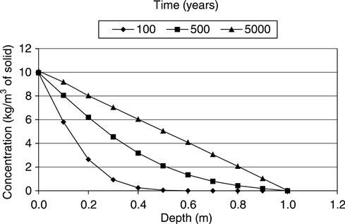
Figure 2.6 shows the effect of changing the capacity factor for each of the examples shown above. It may be seen that this increases the breakthrough time far more effectively than reducing the permeability, which was 10⁻⁹ for the base case and 10⁻¹² for the diffusion control case.

Chapter 15 describes how this model was validated by constructing trial cells, filling them with leachate and extracting samples of pore solution at various depths over a period of three years. With this validation, it was then possible to use the knowledge of the transport properties to predict the performance of the barrier throughout its life. This made it possible to select materials for the concrete which will achieve the containment performance required by the regulatory authorities.

2.5 Conclusions