
13. Using VBA to Create Pivot Tables
IN THIS CHAPTER
Creating a Vanilla Pivot Table in the Excel Interface
Building a Pivot Table in Excel VBA
Using Advanced Pivot Table Features
Using Other Pivot Table Features
Introducing Pivot Tables
Pivot tables are the most powerful tools that Excel has to offer. The concept was first put into practice by Lotus with its Improv product.
I love pivot tables because they are a fast way to summarize massive amounts of data. The name pivot table comes from the ability you have to drag fields in the drop zones and have them recalculate. You can use the basic vanilla pivot table to produce a concise summary in seconds. However, pivot tables come in so many flavors that they can be the tools of choice for many different uses. You can build pivot tables to act as the calculation engine to produce reports by store, by style, or to quickly find the top 5 or bottom 10 of anything.
I am not suggesting you use VBA to build pivot tables to give to your user. I am suggesting you use pivot tables as a means to an end—use a pivot table to extract a summary of data and then take this summary on to better uses.
Understanding Versions
As Microsoft invests in making Excel the premier choice in business intelligence, pivot tables continue to evolve. They were introduced in Excel 5 and perfected in Excel 97. In Excel 2000, pivot table creation in VBA was dramatically altered. Some new parameters were added in Excel 2002. A few new properties such as PivotFilters and TableStyle2 were added in Excel 2007. Slicers and new choices for Show Values As were added in Excel 2010. Therefore, you need to be extremely careful when writing code in Excel 2010 that might be run in legacy versions.
Much of the code in this chapter is backward-compatible all the way to Excel 2000. Pivot table creation in Excel 97 required using the PivotTableWizard method. Although this book will not include code for Excel 97, one example has been included in the sample file for this chapter.
New in Excel 2010
Excel 2010 offers many new features in pivot tables. If you use any of these features in VBA, the code will work in Excel 2010 but crash in any legacy versions of Excel.
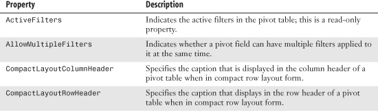
Table 13.1 shows items that are available in Excel 2010 VBA for pivot tables.
Table 13.1. Properties and Methods New in Excel 2010

New Beginning with Excel 2007
If there is some chance that your code will run in Excel 2003, there are even more possible incompatibilities. Many concepts on the Design tab, such as subtotals at the top, the report layout options, blank rows, and the new pivot table styles, were introduced in Excel 2007. Excel 2007 offered better filters than legacy versions of Excel. Every new feature adds one or more methods or properties to VBA.
Caution
If you expect to share your pivot table macro with people running legacy versions of Excel, you need to avoid these methods. Your best bet is to open an Excel 2003 workbook in Compatibility mode and record the macro while the workbook is in Compatibility mode.
Table 13.2 shows the methods that were added in Excel 2007. If you record a macro that uses these methods, you cannot share the macro with someone using a legacy version of Excel.
Table 13.2. Methods That Were New in Excel 2007

Table 13.3 lists the properties that were new in Excel 2007. If you record a macro that refers to these properties, you cannot share the macro with someone using a legacy version of Excel.
Table 13.3. Properties That Were New in Excel 2007


Creating a Vanilla Pivot Table in the Excel Interface
Even though pivot tables are the most powerful feature in Excel, Microsoft estimates they are used by only 7 percent of Excel users overall. Based on surveys at MrExcel.com, about 42 percent of advanced Excel users have used pivot tables. Because a significant portion of Excel users has not used pivot tables, this section walks through the steps of building a pivot table in the user interface.
Let’s say you have 5,000 or 500,000 rows of data, as shown in Figure 13.1. You want a summary of revenue by region and product. Regions should go down the side, products across the top.

Figure 13.1. If you need to summarize 500,000 rows of transactional data quickly, a pivot table can do so in seconds. Your goal is to produce a summary of revenue by region and product.
To build the pivot table to the right of the data, follow these steps:
- Select a single cell in the transaction data. Select the PivotTable icon from the Insert tab. Excel displays the Create PivotTable dialog.
- Verify that Excel filled in the proper address for the table range. Provided your data has no completely blank rows or blank columns, this address is usually correct.
- Select to create the pivot table on an existing worksheet. Click the Location reference box and select Cell J1, as shown in Figure 13.2.

Figure 13.2. Verify that Excel selected the correct data and specify a location for the pivot table.
- Click OK to create a blank pivot table. Instructions in the blank pivot table tell you to choose fields from the PivotTable Field List. The PivotTable Field List appears at the right side of your screen. A list of available fields is in the top of the task pane. The following four drop zones appear at the bottom of the task pane: Report Filter, Column Labels, Row Labels, and Values (see Figure 13.3).
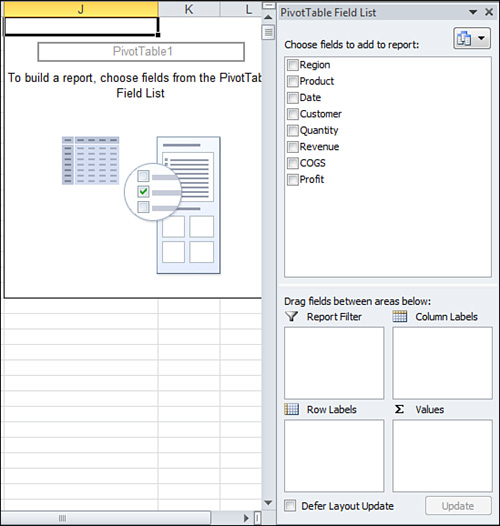
Figure 13.3. Excel presents you with a list of available fields and four drop zones in the PivotTable Field List.
- Click the Region and Revenue fields in the top section of the PivotTable Field List. Because the region field contains text data, it is automatically moved to the Row Labels drop zone. Because Revenue contains numeric data, it is automatically moved to the Values drop zone.
- Click the Product field in the top section of the PivotTable Field List and drag to the Column Labels drop zone in the bottom half of the PivotTable Field List. This adds a list of products stretching across the top row of your pivot table.
Excel has built a concise summary of your data in the pivot table, as shown in Figure 13.4.
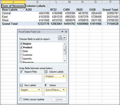
Figure 13.4. Only six clicks were required to create this summary.
After a pivot table has been created on your worksheet, you can easily change the data summarized in the report by dragging fields within the drop zones of the PivotTable Field List. In Figure 13.5, Customer was added to the Row Labels section of the existing pivot table.
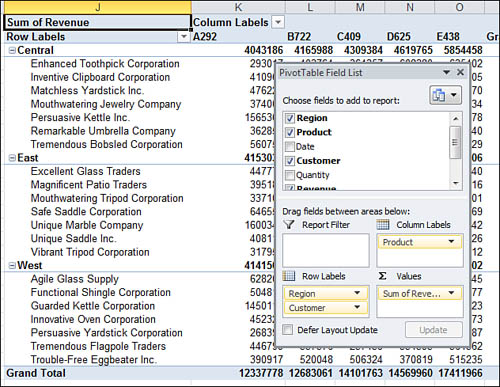
Figure 13.5. In a couple of clicks, you can move Region across the top, move Product down the side, and add a summary by Customer.
Understanding Compact Layout
Beginning with Excel 2007, all pivot tables created in the Excel interface are created in a new layout called Compact Form. In this layout, multiple Row fields appear in a single column at the left of the pivot table. Excel also puts the subtotals above the detail rows.
Although these changes might make for a better live pivot table, most of the pivot tables in this chapter will be converted to values to produce a static summary of the data. In these cases, you want to perform the following steps in the user interface:
- On the Design tab, select Report Layout, Show in Tabular Form, and then select Repeat All Item Labels.
- On the Design tab, select Subtotals, Do Not Show Subtotals.
- On the Options tab, select the Options icon on the left side of the ribbon. In the Layout & Format tab of the PivotTable Options dialog, type a
0next to For Empty Cells Show. - On the Design tab, select Grand Totals, Off for Rows and Columns.
After implementing these changes, you will have a solid, contiguous block of data, as shown in Figure 13.6.

Figure 13.6. If you plan to reuse the output of the pivot table for further analysis, a few changes to the default settings are required.
Building a Pivot Table in Excel VBA
This chapter does not mean to imply that you should use VBA to build pivot tables to give to your clients. Instead, the purpose of this chapter is to remind you that pivot tables can be used as a means to an end; you can use a pivot table to extract a summary of data and then use that summary elsewhere.
Note
The code listings from this chapter are available for download at http://www.MrExcel.com/getcode2010.html.
Caution
Although the Excel user interface has new names for the various sections of a pivot table, VBA code continues to refer to the old names. Microsoft had to use this choice; otherwise, millions of lines of code would stop working in Excel 2007 when they referred to a page field rather than a filter field. Although the four sections of a pivot table in the Excel user interface are Report Filter, Column Labels, Row Labels, and Values, VBA continues to use the old terms of Page fields, Column fields, Row fields, and Data fields.
Defining the Pivot Cache
In Excel 2000 and later, you first build a pivot cache object to describe the input area of the data:

Creating and Configuring the Pivot Table
After defining the pivot cache, use the CreatePivotTable method to create a blank pivot table based on the defined pivot cache:
Set PT = PTCache.CreatePivotTable(TableDestination:=WSD.Cells(2, _
FinalCol + 2), TableName:="PivotTable1")
In the CreatePivotTable method, you specify the output location and optionally give the table a name. After running this line of code, you have a strange-looking blank pivot table, like the one shown in Figure 13.7. You now have to use code to drop fields onto the table.
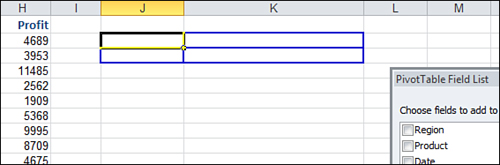
Figure 13.7. When you use the CreatePivotTable method, Excel gives you a four-cell blank pivot table that is not very useful.
If you choose the Defer Layout Update setting in the user interface to build the pivot table, Excel does not recalculate the pivot table after you drop each field onto the table. By default in VBA, Excel calculates the pivot table as you execute each step of building the table. This could require the pivot table to be executed a half-dozen times before you get the final result. To speed up your code execution, you can temporarily turn off calculation of the pivot table by using the ManualUpdate property:
PT.ManualUpdate = True
You can now run through the steps needed to lay out the pivot table. In the .AddFields method, you can specify one or more fields that should be in the row, column, or filter area of the pivot table.
The RowFields parameter enables you to define fields that appear in the Row Labels drop zone of the PivotTable Field List. The ColumnFields parameter corresponds to the Column Labels drop zone. The PageFields parameter corresponds to the Report Filter drop zone.
The following line of code populates a pivot table with two fields in the row area and one field in the column area:
' Set up the row & column fields
PT.AddFields RowFields:=Array("Region", "Customer"), _
ColumnFields:="Product"
To add a field such as Revenue to the values area of the table, you change the Orientation property of the field to be xlDataField.
Adding Fields to the Data Area
When you are adding fields to the Data area of the pivot table, there are many settings you should control instead of letting Excel’s intellisense decide.
For example, say you are building a report with revenue in which you will likely want to sum the revenue. If you don’t explicitly specify the calculation, Excel scans through the data in the underlying data. If 100 percent of the revenue columns are numeric, Excel will sum those columns. If one cell is blank or contains text, Excel will decide on that day to count the revenue, which will produce confusing results.
Because of this possible variability, you should never use the DataFields argument in the AddFields method. Instead, change the property of the field to xlDataField. You can then specify the Function to be xlSum.
While you are setting up the data field, you can change several other properties within the same With...End With block.
The Position property is useful when adding multiple fields to the data area. Specify 1 for the first field, 2 for the second field, and so on.
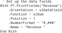
By default, Excel will rename a Revenue field to have a strange name like Sum of Revenue. You can use the .Name property to change that heading back to something normal.
Tip
Note that you cannot reuse the word “Revenue” as a name. Instead, you should use “Revenue” (with a space).
You are not required to specify a number format, but it can make the resulting pivot table easier to understand, and only takes an extra line of code.
At this point, you have given VBA all the settings required to generate the pivot table correctly. If you set ManualUpdate to False, Excel calculates and draws the pivot table. You can immediately thereafter set this back to True:
' Calc the pivot table
PT.ManualUpdate = False
PT.ManualUpdate = True
Your pivot table inherits the table style settings selected as the default on whatever computer happens to run the code. If you want control over the final format, you can explicitly choose a table style. The following code applies banded rows and a medium table style:
' Format the pivot table
PT.ShowTableStyleRowStripes = True
PT.TableStyle2 = "PivotStyleMedium10"
If you want to reuse the data from the pivot table, turn off the grand totals and subtotals and fill in the labels along the left column. For an explanation of why this code turns off the subtotals, see “Suppressing Subtotals for Multiple Row Fields” near the end of this chapter.

At this point, you have a complete pivot table like the one shown in Figure 13.8.
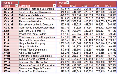
Figure 13.8. Fewer than 50 lines of code created this pivot table in less than a second.
Listing 13.1 shows the complete code used to generate the pivot table.
Listing 13.1. Code to Generate a Pivot Table


Learning Why You Cannot Move or Change Part of a Pivot Report
Although pivot tables are incredible, they have annoying limitations; for example, you cannot move or change just part of a pivot table. Try to run a macro that clears Row 2. The macro comes to a screeching halt with an error 1004, as shown in Figure 13.9. To get around this limitation, you can copy the pivot table and paste as values.
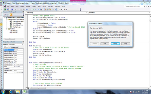
Figure 13.9. You cannot delete just part of a pivot table.
Determining Size of a Finished Pivot Table to Convert the Pivot Table to Values
Knowing the size of a pivot table in advance is difficult. If you run a report of transactional data on one day, you may or may not have sales from the West region, for example. This could cause your table to be either six or seven columns wide. Therefore, you should use the special property TableRange2 to refer to the entire resultant pivot table.
PT.TableRange2 includes the entire pivot table. In Figure 13.10, TableRange2 includes the extra row at the top with the button Sum of Revenue. To eliminate that row, the code copies PT.TableRange2 but offsets this selection by one row by using .Offset(1, 0). Depending on the nature of your pivot table, you might need to use an offset of two or more rows to get rid of extraneous information at the top of the pivot table.

Figure 13.10. This figure shows an intermediate result of the macro. Only the summary in J12:M17 will remain after the macro finishes.
The code copies PT.TableRange2 and uses PasteSpecial on a cell five rows below the current pivot table. At that point in the code, your worksheet appears as shown in Figure 13.10. The table in J2 is a live pivot table, and the table in J12 is just the copied results.
You can then eliminate the pivot table by applying the Clear method to the entire table. If your code is then going on to do additional formatting, you should remove the pivot cache from memory by setting PTCache equal to Nothing.
The code in Listing 13.2 uses a pivot table to produce a summary from the underlying data. At the end of the code, the pivot table will be copied to static values and the pivot table will be cleared.
Listing 13.2. Code to Produce a Static Summary from a Pivot Table


The code in Listing 13.2 creates the pivot table. It then copies the results and pastes them as values in J12:M13. Figure 13.10, which was shown previously, includes an intermediate result just before the original pivot table is cleared.
So far, this chapter has walked you through building the simplest of pivot table reports. Pivot tables offer far more flexibility. The sections that follow present more complex reporting examples.
Using Advanced Pivot Table Features
In this section, you will take the detailed transactional data and produce a series of reports for each product line manager. This section covers the following advanced pivot table features that are required in these reports:
• Group the daily dates up to yearly dates
• Add multiple fields to the value area
• Control the sort order so the largest customers are listed first
• Use the ShowPages feature to replicate the report for each product line manager
• After producing the pivot tables, convert the pivot table to values and do some basic formatting
Figure 13.11 shows the report for one product line manager so that you can understand the final goal.

Figure 13.11. Using pivot tables simplifies the creation of the report.
Using Multiple Value Fields
The report has three fields in the values area; Count of Orders, Revenue, and % of Total Revenue. Anytime you have two or more fields in the values area, a new virtual field named Data becomes available in your pivot table.
In Excel 2010, this field appears as sigma values in the drop zone of the Pivot Table Field List. When creating your pivot table, you can specify Data as one of the column fields or row fields.
The position of the Data field is important. It usually works best as the innermost column field.
When you define your pivot table in VBA, you will have two columns fields: the Date field and the Data field. To specify two or more fields in the AddFields method, you wrap those fields in an array function.
Use this code to define the pivot table:
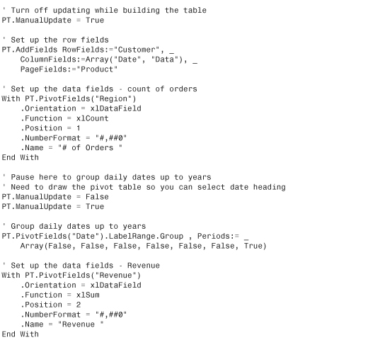
' Set up the row fields
PT.AddFields RowFields:="Customer", _
ColumnFields:=Array("Date", "Data"), _
PageFields:="Product"
This is the first time you have seen the PageFields parameter in this chapter. If you were creating a pivot table for someone to use, the fields in the PageField allow for easy ad hoc analysis. In this case, the value in the PageField is going to make it easy to replicate the report for every product line manager.
Counting the Number of Records
So far, the .Function property of the data fields has always been .xlSum. There are a total of 11 functions available: xlSum, xlCount, xlAverage, xlStdDev, xlMin, xlMax, and so on.
Count is the only function that works for text fields. To count the number of records, and hence the number of orders, add a text field to the data area and choose .xlCount as the function.
With PT.PivotFields("Region")
.Orientation = xlDataField
.Function = xlCount
.Position = 1
.NumberFormat = "#,##0"
.Name = "# of Orders "
End With
Caution
This is a count of the number of records. It is not a count of the distinct values in a field. This has always been difficult to do in a pivot table. It is now fairly easy to do with the PowerPivot add-in. Unfortunately, you cannot use VBA to build a PowerPivot pivot table.
Grouping Daily Dates to Months, Quarters, or Years
Pivot tables have the amazing ability to group daily dates up to months, quarters, and/or years. In VBA, this feature is a bit annoying because you must select a date cell before issuing the command. As you saw in Figure 13.10, your pivot table usually stays as four blank cells until the end of the macro, so there really is not a date field to select.
However, if you need to group a date field, you will have to let the pivot table redraw. To do this, use this code:
' Pause here to group daily dates up to years
' Need to draw the pivot table so you can select date heading
PT.ManualUpdate = False
PT.ManualUpdate = True
Tip
I used to go through all sorts of gyrations to figure out where the first date field was. In fact, you can simply refer to PT.PivotFields("Date").LabelRange to point to the date heading.
There are seven ways to group times or dates: Seconds, Minutes, Hours, Days, Months, Quarters, and Years. Note that you can group a field by multiple items. You specify a series of seven True/False values corresponding to Seconds, Minutes, and so on.
For example, to group by Months, Quarters, and Years, you would use the following:
PT.PivotFields("Date").LabelRange.Group , Periods:= _
Array(False, False, False, False, True, True, True)
Caution
Never choose to group by only months without including years. If you do this, Excel combines January from this year and January from last year into a single item called January. Although this is great for seasonality analyses, it is rarely what you want in a summary. Always choose Years and Months in the Grouping dialog.
If you want to group by week, you group only by day and use 7 as the value for the By parameter:
![]()
Specifying True for Start and End will start the first week at the earliest date in the data. If you only want to show weeks starting from Monday January 3, 2011 through Sunday January 1, 2012, use this code:

![]() To see a demo of grouping by week, search for Excel VBA 13 at YouTube.
To see a demo of grouping by week, search for Excel VBA 13 at YouTube.
Caution
There is one limitation to grouping by week. When you group by week, you cannot also group by any other measure. For example, grouping by week and quarter is not valid.
For this report, you only need to group by year, so the code is as follows:
![]()
Caution
Before grouping the daily dates up to years, you had about 500 date columns across this report. After grouping, you have two date columns plus a total. I prefer to group the dates as soon as possible in the macro. If you added the other two data fields to the report before grouping, your report would be 1500 columns wide. While this is not a problem since Excel 2007 increased the column limit from 256 to 16,384, it still creates an unusually large report when you ultimately only need a few columns.
Figure 13.12 shows the report before grouping the dates up to years. Figure 13.13 shows the report after grouping to years.

Figure 13.12. Five hundred daily dates stretch across the report.
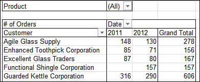
Figure 13.13. After one line of code, the dates are rolled up to years.
Note
After you issue this command, the years field is still called Date. This may not always be true. If you roll daily dates up to months and to years, the Date field will contain months, and a new Year field will be added to the field list to hold years.
Changing the Calculation to Show Percentages
Excel 2010 offers a new Show Values As drop-down in the Options tab. Although some of the options in that drop-down are truly new to Excel 2010, most of the options have been hidden away on a back tab of the Field Settings dialog.
These calculations allow you to change how a field is displayed in the report. Instead of showing sales, you could show the sales as a percentage of the total sales. You could show a running total. You could show each day’s sales as a percentage of the previous day’s sales.
All these settings are controlled through the .Calculation property of the pivot field. Each calculation has its own unique set of rules. Some, such as % of column, work without any further settings. Others, such as Running Total In, require a base field. Others, such as running total, require a base field and a base item.
To get the percentage of the total, specify xlPercentOfTotal as the .Calculation property for the page field:
.Calculation = xlPercentOfTotal
To set up a running total, you have to specify a BaseField. Say that you need a running total along a date column:
' Set up Running Total
.Calculation = xlRunningTotal
.BaseField = "Date"
With ship months going down the columns, you might want to see the percentage of revenue growth from month to month. You can set up this arrangement with the xlPercentDifferenceFrom setting. In this case, you must specify that the BaseField is "Date" and that the BaseItem is something called (previous):
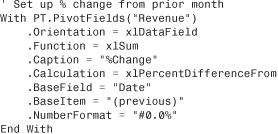
Note that with positional calculations, you cannot use the AutoShow or AutoSort method. This is too bad; it would be interesting to sort the customers high to low and to see their sizes in relation to each other.
You can use the xlPercentDifferenceFrom setting to express revenues as a percentage of the West region sales:
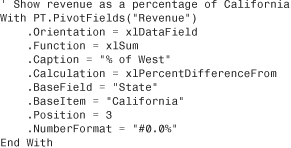
Table 13.4 shows the complete list of .Calculation options. The second column indicates whether the calculation is compatible with earlier versions of Excel. The third column indicates if you need a base field and base item.
Table 13.4. Complete List of .Calculation Options

After that long explanation of the .Calculation property, you can build the other two pivot table fields for the product line report.
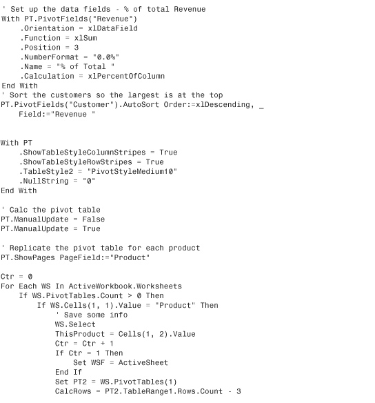
Add Revenue to the report twice. The first time, there is no calculation. The second time, calculate the percentage of total:
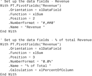
Tip
Take careful note of the name of the first field above. By default, Excel would use Sum of Revenue. Like me, if you think this is a goofy title, you can change it. However, you cannot change it to Revenue because there is already a field in the pivot table field list with that name.
In the preceding code, I used the name “Revenue” (with a trailing space). This works fine, and no one notices the extra space. However, in the rest of the macro, when you refer to this field, remember to refer to it as “Revenue” (with a trailing space).
Eliminating Blank Cells in the Values Area
If you have some customers who were new in year 2, their sales will appear blank in year 1. Anyone using Excel 97 or later can replace blank cells with zeros. In the Excel interface, you can find the setting on the Layout & Format tab of the PivotTable Options dialog box. Select the For Empty Cells, Show option and type 0 in the box.
The equivalent operation in VBA is to set the NullString property for the pivot table to "0":
PT.NullString = "0"
Note
Although the proper code is to set this value to a text zero, Excel actually puts a real zero in the empty cells.
Controlling the Sort Order with AutoSort
The Excel interface offers an AutoSort option that enables you to show customers in descending order based on revenue. The equivalent code in VBA to sort the product field by descending revenue uses the AutoSort method:
PT.PivotFields("Customer").AutoSort Order:=xlDescending, _
Field:="Revenue "
After applying some formatting in the macro, you now have one report with totals for all products, as shown in Figure 13.14.

Figure 13.14. Replicate this report for each product.
Replicating the Report for Every Product
As long as your pivot table was not built on an OLAP data source, you now have access to one of the most powerful, but least-well-known features in pivot tables. The command is called Show Report Filter Pages, and it will take your pivot table and replicate it for every item in one of the fields in the Report Filter area.
Because you built the report with Product as a filter field, it takes only one line of code to replicate the pivot table for every product.
' Replicate the pivot table for each product
PT.ShowPages PageField:="Product"
After running this line of code, you will have a new worksheet for every product in the dataset.
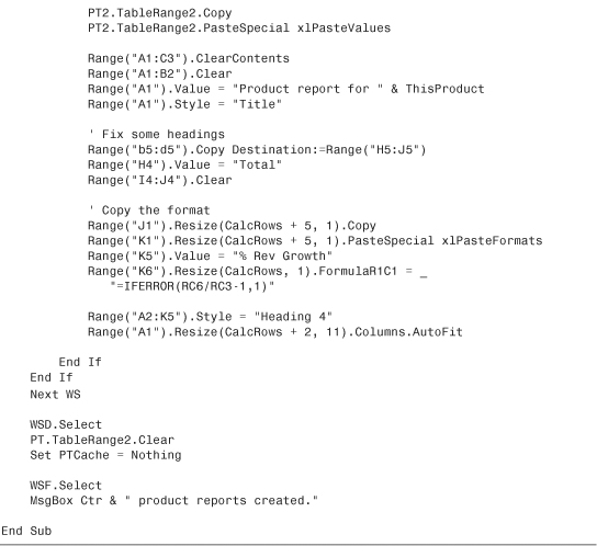
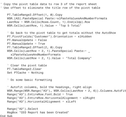
From there, you have some simple formatting and calculations. Check the end of the macro for these techniques, which should be second nature by this point in the book.
Listing 13.3 shows the complete macro.
Listing 13.3. The Complete Macro

Filtering a Data Set
There are many ways to filter a pivot table, from the new Excel 2010 slicers, to the Excel 2007 conceptual filters, to simply selecting and clearing items from one of the many field drop-downs.
Manually Filtering Two or More Items in a Pivot Field
When you open a field heading drop-down and select or clear items from the list, you are applying a manual filter.

Figure 13.15. This filter drop-down offers manual filters, a search box, and conceptual filters.
For example, you have one client who sells shoes. In the report showing sales of sandals, he wants to see just the stores that are in warm-weather states. The code to hide a particular store is as follows:
PT.PivotFields("Store").PivotItems("Minneapolis").Visible = False
This process is easy in VBA. After building the table with Product in the page field, loop through to change the Visible property to show only the total of certain products:

Using the Conceptual Filters
Excel 2007 introduced new conceptual filters for date fields, numeric fields, and text fields. Open the drop-down for any field label in the pivot table. In the drop-down that appears, you can choose Label Filters, Date Filters, or Value Filters. The Date filters offer the ability to filter to a conceptual period such as last month or next year (see Figure 13.16).
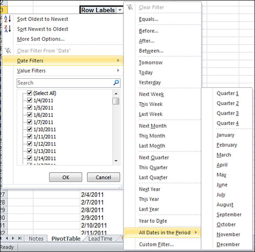
Figure 13.16. These date filters were introduced in Excel 2007.
To apply a label filter in VBA, use the PivotFilters.Add method. The following code filters to the customers that start with the letter E:
PT.PivotFields("Customer").PivotFilters.Add _
Type:=xlCaptionBeginsWith, Value1:="E"
To clear the filter from the Customer field, use the ClearAllFilters method:
PT.PivotFields("Customer").ClearAllFilters
To apply a date filter to the date field to find records from this week, use this code:
PT.PivotFields("Date").PivotFilters.Add Type:=xlThisWeek
The value filters allow you to filter one field based on the value of another field. For example, to find all the markets where the total revenue is over $100,000, you would use this code:
PT.PivotFields("Market").PivotFilters.Add _
Type:=xlValueIsGreaterThan, _
DataField:=PT.PivotFields("Sum of Revenue"), _
Value1:=100000
Other value filters might allow you to specify that you want branches where the revenue is between $50,000 and $100,000. In this case, you would specify one limit as Value1 and the second limit as Value2:
PT.PivotFields("Market").PivotFilters.Add _
Type:=xlValueIsBetween, _
DataField:=PT.PivotFields("Sum of Revenue"), _
Value1:=50000, Value2:=100000
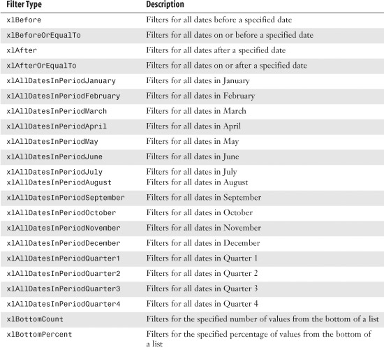
Table 13.5 lists all the possible filter types.
Table 13.5. Filter Types


Using the Search Filter
Excel 2010 added a Search box to the filter drop-down. While this is a slick feature in the Excel interface, there is no equivalent magic in VBA. Whereas the drop-down offers the Select All Search Results check box, the equivalent VBA just lists all the items that match the selection.
There is nothing new in Excel 2010 VBA to emulate the search box. To achieve the same results in VBA, use the xlCaptionContains filter described in the previous style.
Case Study: Filtering to Top Five or Top 10 Using a Filter
If you are designing an executive dashboard utility, you might want to spotlight the top five customers. As with the AutoSort option, you could be a pivot table pro and never have stumbled across the Top 10 AutoShow feature in Excel. This setting lets you select either the top or the bottom n records based on any Data field in the report.
The code to use AutoShow in VBA uses the .AutoShow method:
![]()
When you create a report using the .AutoShow method, it is often helpful to copy the data and then go back to the original pivot report to get the totals for all markets. In the code, this is achieved by removing the Customer field from the pivot table and copying the grand total to the report. The code produces the report shown in Figure 13.17.

Figure 13.17. The Top 5 Customers report contains two pivot tables.


The Top 5 Customers report actually contains two snapshots of a pivot table. After using the AutoShow feature to grab the top five markets with their totals, the macro went back to the pivot table, removed the AutoShow option, and grabbed the total of all customers to produce the Total Company row.
Setting Up Slicers to Filter a Pivot Table
Excel 2010 introduced the concept of slicers to filter a pivot table. A slicer is a visual filter. Slicers can be resized and repositioned. You can control the color of the slicer and control the number of columns in a slicer. You can also select or unselect items from a slicer using VBA.
Figure 13.18 shows a pivot table with five slicers. The Date slicer has been modified to have three columns.

Figure 13.18. Slicers provide a visual filter of several fields.
A slicer consists of a slicer cache and a slicer. To define a slicer cache, you need to specify a pivot table as the source and a field name as the SourceField. The slicer cache is defined at the workbook level. This would allow you to have the slicer on a different worksheet than the actual pivot table:

After you have defined the slicer cache, you can add the slicer. The slicer is defined as an object of the slicer cache. Specify a worksheet as the destination. The name argument controls the internal name for the slicer. The Caption argument is the heading that will be visible in the slicer. This might be useful if you would like to show the name Region, but the IT department defined the field as IDKRegn. Specify the size of the slicer using height and width in points. Specify the location using top and left in point.
In the followimg code, the values for top, left, height, and width are assigned to be equal to the location or size of certain cell ranges:

All slicers start out as one column. You can change the style and number of columns with this code:

I find that when I create slicers in the Excel interface, I spend many mouse clicks making adjustments to the slicers. After adding two or three slicers, they are arranged in an overlapping tile arrangement. I always tweak the location, size, number of columns, and so on. In my seminars, I always brag that I can create a complex pivot table in six mouse clicks. Slicers are admittedly powerful but seem to take 20 mouse clicks before they look right. Having a macro make all of these adjustments at once is a time-saver.
Once the slicer is defined, you can actually use VBA to choose which items are activated in the slicer. It seems counter-intuitive, but to choose items in the slicer, you have to change the SlicerItem, which is a member of the SlicerCache, not a member of the Slicer:
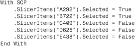
You might need to deal with slicers that already exist. If a slicer is created for the product field, the name of the SlicerCache will be "Slicer_Product". The following code will format existing slicers:

Filtering an OLAP Pivot Table Using Named Sets
Ready for some good news, bad news, and sneaky news?
Good News: Named Sets
Microsoft added an amazing feature to Excel 2010 pivot tables called named sets. This feature allows you to create filters that were never possible before. For example, in Figure 13.19, the pivot table shows Actuals and Budget for FY2009 and FY2010. It would have been impossible to show an asymmetric report with only FY2009 Actuals and FY 2010 Budget: when you turned off Budget for 2009, it would have been turned off for all years. Named sets allow you to overcome this.

Figure 13.19. You want to show 2009 Actuals and 2010 Budget.
Bad News Named Sets Limitations
Named sets only work for data coming from OLAP pivot tables. If you are dealing with pivot tables based on regular Excel data, you will have to wait until a future release of Excel to tap into the power of named sets.
Sneaky News: Workaround
A pivot table produced using the PowerPivot add-in is actually an OLAP pivot table. To create the pivot table shown in Figure 13.19, I copied the Excel data, pasted as a new table in the PowerPivot add-in, and then returned to Excel to create the pivot table.
Note
PowerPivot is a free add-in for Excel 2010 brought to you by the SQL Server Analysis Services team at Microsoft. Because you cannot control PowerPivot from VBA, it is not covered in this book. However, it is a great add-in. You can use PowerPivot to mash up datasets from multimillion row datasets. You can use PowerPivot to define calculations not possible in regular Excel pivot tables. I have written an entire book about PowerPivot: PowerPivot for the Excel Data Analyst.
This is a minor use for a powerful tool. The PowerPivot add-in is designed to mash-up multimillion row recordsets from various sources. To take a single flat table and paste it into the powerful tool is admittedly underutilizing the tool. However, it is one great way to get an unbalanced pivot table report.
Using a Named Set for Asymmetric Pivot Table
A common request is to show an asymmetric selection from two column fields. In Figure 13.19, you would like to show 2009 year’s actual and 2010 budget.
To define a named set, you will have to build a formula that uses the MDX language. MDX stands for Multidimensional Expressions Language. There are many MDX tutorials on the Internet. Luckily, you can turn on the macro recorder while you define a named set using the Excel 2010 interface and have the macro recorder write the MDX formula for you.
When you are defining a named set, you will define both a CalculatedMember and then add a CubeField set. These declarations at the top of the macro will initialize two calculated members:
Dim CM1 As CalculatedMember
The MDX formula is the key to the named set. In this code, the formula contains 2009 Actuals and 2010 Budget. The formula starts and ends with curly braces indicating that the formula contains an array of values. Each line of code is adding another column to the array:
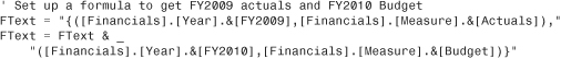
After you have defined the formula, use the following code to add the calculated member to the dataset:
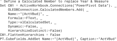
This code will add a new folder to the pivot table field list called Sets. In that folder, an item called ActVBud will be available as field, just like the field called Year or Measure. In your code, you will want to replace the Year and Measure field in the pivot table with the ActVBud field:

Figure 13.20 shows the asymmetric report.
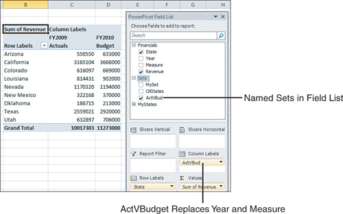
Figure 13.20. Named sets enable asymmetric reporting.
Using Other Pivot Table Features
This section covers a few additional features in pivot tables that you might need to code with VBA.
Calculated Data Fields
Pivot tables offer two types of formulas. The most useful type defines a formula for a calculated field. This adds a new field to the pivot table. Calculations for calculated fields are always done at the summary level. If you define a calculated field for average price as revenue divided by units sold, Excel first adds the total revenue and total quantity, and then it does the division of these totals to get the result. In many cases, this is exactly what you need. If your calculation does not follow the associative law of mathematics, it might not work as you expect.
To set up a Calculated field, use the Add method with the CalculatedFields object. You have to specify a field name and a formula.
Note
Note that if you create a field called Profit Percent, the default pivot table produces a field called Sum of Profit Percent. This title is misleading and downright silly. The solution is to use the Name property when defining the Data field to replace Sum of Profit Percent with something such as GP Pct. Keep in mind that this name must differ from the name for the Calculated field.

Calculated Items
Suppose you have a Measure field with two items, Budget and Actual. You would like to add a new position to calculate Variance as Actual-Budget. You can do this with a calculated item by using this code:
![]()
Using ShowDetail to Filter a Recordset
When you take any pivot table in the Excel user interface and then double-click any number in the table, Excel will insert a new sheet in the workbook and copies all the source records that represent that number. In the Excel user interface, this is a great way to perform a drill-down query into a dataset.
The equivalent VBA property is ShowDetail. By setting this property to True for any cell in the pivot table, you generate a new worksheet with all the records that make up that cell:
PT.TableRange2.Offset(2, 1).Resize(1, 1).ShowDetail = True
Changing the Layout from the Design Tab
The Layout group of the Design tab contains four drop-downs that control the following:
• Location of subtotals (top or bottom)
• Presence of grand totals
• Report layout including if outer row labels are repeated
• Presence of blank rows
Subtotals can appear either at the top or at the bottom of a group of pivot items. The SubtotalLocation property applies to the entire pivot table; valid values are xlAtBottom or xlAtTop:
PT.SubtotalLocation:=xlAtTop
Grand totals can be turned on or off for rows or columns. Because these two settings can be confusing, remember that at the bottom of a report, there is a total line that most people would call the Grand Total Row. To turn off that row, you have to use the following:
PT.ColumnGrand = False
You need to turn off the ColumnGrand when you want to suppress the total row because Microsoft calls that row the “grand total for columns.” Get it? In other words, they are saying that the row at the bottom contains the total of the columns above it. I finally started doing better when I would decide which one to turn off, and then turn off the opposite one.
To suppress what you would call the Grand Total Column along the right side of the report, you have to suppress what Microsoft calls the Total for Rows with the following code:
PT.RowGrand = False
Settings for the Report Layout
There are three settings for the report layout.
• Tabular layout—Similar to the default layout in Excel 2003
• Outline layout—Optionally available in Excel 2003
• Compact layout—Introduced in Excel 2007
When you create a pivot table in the Excel interface, you will get compact layout. When you build a pivot table in VBA, you will get the tabular layout. You can change to one of the other layouts with one of these lines:
PT.RowAxisLayout xlTabularRow
PT.RowAxisLayout xlOutlineRow
PT.RowAxisLayout = xlCompactRow
Starting in Excel 2007, you can add a blank line to the layout after each group of pivot items. Although the Design tab offers a single setting to affect the entire pivot table, the setting is actually applied to each individual pivot field individually. The macro recorder responds by recording a dozen lines of code for a pivot table with 12 fields. You can intelligently add a single line of code for the outer Row fields:
PT.PivotFields("Region").LayoutBlankLine = True
Suppressing Subtotals for Multiple Row Fields
As soon as you have more than one row field, Excel automatically adds subtotals for all but the innermost row field. That extra row field can get in the way if you plan on reusing the results of the pivot table as a new dataset for some other purpose. Although accomplishing this task manually can be relatively simple, the VBA code to suppress subtotals is surprisingly complex.
Most people do not realize that it is possible to show multiple types of subtotals. For example, you can choose to show Total, Average, Min, and Max in the same pivot table.
To suppress subtotals for a field, you must set the Subtotals property equal to an array of 12 False values. The first False turns off automatic subtotals, the second False turns off the Sum subtotal, the third False turns off the Count subtotal, and so on. This line of code suppresses the Region subtotal:
PT.PivotFields("Region").Subtotals = Array(False, False, False, False, _
False, False, False, False, False, False, False, False)
A different technique is to turn on the first subtotal. This method automatically turns off the other 11 subtotals. You can then turn off the first subtotal to make sure that all subtotals are suppressed:
PT.PivotFields("Region").Subtotals(1) = True
PT.PivotFields("Region").Subtotals(1) = False
Case Study: Applying a Data Visualization
Beginning with Excel 2007, fantastic data visualizations such as icon sets, color gradients, and in-cell data bars are offered. When you apply visualization to a pivot table, you should exclude the total rows from the visualization.
If you have 20 customers that average $3,000,000 in revenue each, the total for the 20 customers is $60 million. If you include the total in the data visualization, the total gets the largest bar, and all the customer records have tiny bars.
In the Excel user interface, you always want to use the Add Rule or Edit Rule choice to select the option All Cells Showing “Sum of Revenue” for “Customer.”
The code to add a data bar to the Revenue field is as follows:

Next Steps
If you cannot already tell, pivot tables are my favorite feature in Excel. They are incredibly powerful and flexible. Combined with VBA, they provide an excellent calculation engine and power many of the reports I build for clients. In Chapter 14, “Excel Power,” you learn multiple techniques for handling various tasks in VBA.