14. Excel Power
A major secret of successful programmers is to never waste time writing the same code twice. They all have little bits—or even big bits—of code that are used over and over again. Another big secret is to never take 8 hours doing something that can be done in 10 minutes—which is what this book is about!
This chapter contains programs donated by several Excel power programmers. These are programs they have found useful, and they hope these will help you too. Not only can they save you time, but they may also teach you new ways of solving common problems.
Different programmers have different programming styles, and we did not rewrite the submissions. As you review the lines of code, you will notice different ways of doing the same task such as referring to ranges.
File Operations
The following utilities deal with handling files in folders. Being able to loop through a list of files in a folder is a useful task.
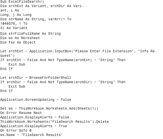
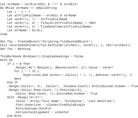
List Files in a Directory
Submitted by Nathan P. Oliver of Minneapolis, Minnesota. Nathan is a financial consultant and application developer.
This program returns the filename, size, and date modified of all specified file types in the selected directory and its subfolders.


Import CSV
Submitted by Masaru Kaji of Kobe-City, Japan. Masaru provides Excel consultation through Colo’s Excel Junk Room (www.puremis.net/excel).
If you find yourself importing a lot of comma-separated variable (CSV) files and then having to go back and delete them, this program is for you. It quickly opens a CSV in Excel and permanently deletes the original file:

Read Entire TXT to Memory and Parse
Submitted by Suat Mehmet Ozgur of Istanbul, Turkey. Suat develops applications in Excel, Access, and Visual Basic.
This sample takes a different approach to reading a text file. Instead of reading one record at a time, the macro loads the entire text file into memory in a single string variable. The macro then parses the string into individual records. The advantage of this method is that you access the file on disk only one time. All subsequent processing occurs in memory and is very fast:


Combining and Separating Workbooks
The next four utilities demonstrate how to combine worksheets into single workbooks or separate a single workbook into individual worksheets or Word documents.
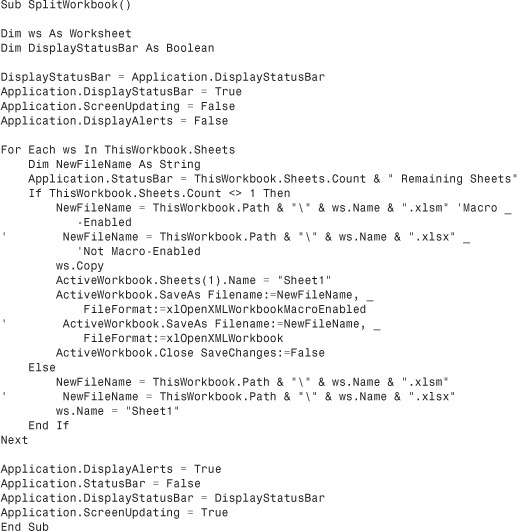
Separate Worksheets into Workbooks
Submitted by Tommy Miles of Houston, Texas.
This sample goes through the active workbook and saves each sheet as its own workbook in the same path as the original workbook. It names the new workbooks based on the sheet name, and it will overwrite files without prompting. You will also notice that you need to choose whether you save the file as XLSM (macro-enabled) or XLSX (macros will be stripped). In the following code, both lines are included—xlsm and xlsx—but the xlsx lines are commented out, making them inactive:
Combine Workbooks
Submitted by Tommy Miles.
This sample goes through all the Excel files in a specified directory and combines them into a single workbook. It renames the sheets based on the name of the original workbook:

Filter and Copy Data to Separate Worksheets
Submitted by Dennis Wallentin of Ostersund, Sweden. Dennis provides Excel tips and tricks at www.xldennis.com.
This sample uses a specified column to filter data and copies the results to new worksheets in the active workbook:

Export Data to Word
Submitted by Dennis Wallentin.
This program transfers data from Excel to the first table found in a Word document. It uses early binding, so a reference must be established in the VB Editor using Tools, References to the Microsoft Word object library:


Working with Cell Comments
Cell comments are often underused features of Excel. The following four utilities help you to get the most out of cell comments.
List Comments
Submitted by Tommy Miles.
Excel allows the user to print the comments in a workbook, but it does not specify the workbook or worksheet on which the comments appear, only the cell, as shown in Figure 14.1.

Figure 14.1. Excel prints only the origin cell address and its comment.
The following sample places comments, author, and location of each comment on a new sheet for easy viewing, saving, or printing. Figure 14.2 shows a sample result.

Figure 14.2. Easily list all the information pertaining to comments.


Resize Comments
Submitted by Tom Urtis of San Francisco, California. Tom is the principal owner of Atlas Programming Management, an Excel consulting firm in the Bay Area.
Excel doesn’t automatically resize cell comments. In addition, if you have several on a sheet, as shown in Figure 14.3, it can be a hassle to resize them one at a time. The following sample code resizes all the comment boxes on a sheet so that, when selected, the entire comment is easily viewable, as shown in Figure 14.4.

Figure 14.3. By default, Excel doesn’t size the comment boxes to show all the entered text.

Figure 14.4. Resize the comment boxes to fit all the text.

Resize Comments with Centering
Submitted by Tom Urtis.
This sample resizes all the comment boxes on a sheet by centering the comments (see Figure 14.5).

Figure 14.5. Center all the comments on a sheet.

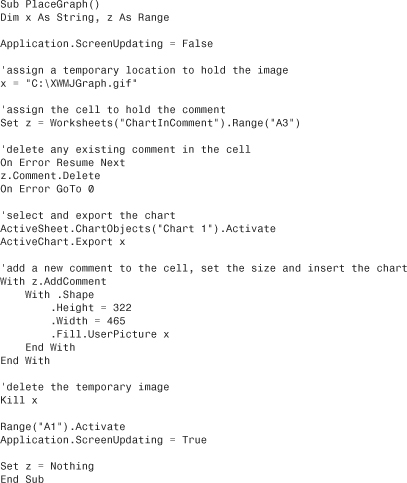
Place a Chart in a Comment
Submitted by Tom Urtis.
A live chart cannot exist in a shape, but you can take a picture of the chart and load it into the comment shape, as shown in Figure 14.6.

Figure 14.6. Place a chart in a cell comment.
The steps to do this manually are as follows:
- Create and save the picture image you want the comment to display.
- If you have not already done so, create the comment and select the cell in which the comment is located.
- From the Review tab, select Edit Comment, or right-click the cell and select Edit Comment.
- Right-click the comment border and select Format Comment.
- Select the Colors and Lines tab, and click the down arrow belonging to the Color field of the Fill section.
- Select Fill Effects, select the Picture tab, and then click the Select Picture button.
- Navigate to your desired image, select the image, and click OK twice.
The effect of having a “live chart” in a comment can be achieved if, for example, the code is part of a SheetChange event when the chart’s source data is being changed. In addition, business charts are updated often, so you might want a macro to keep the comment updated and to avoid repeating the same steps.
The following macro does just that—it modifies the macro for file path name, chart name, destination sheet, cell, and size of comment shape, depending on the size of the chart:
Utilities to Wow Your Clients
The next four utilities will amaze and impress your clients.
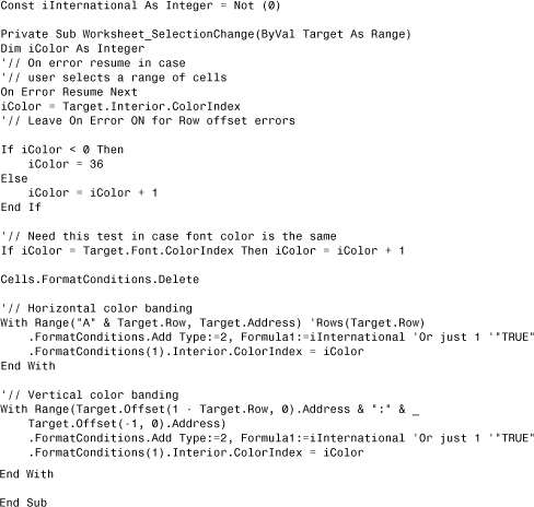
Using Conditional Formatting to Highlight Selected Cell
Submitted by Ivan F. Moala of Auckland, New Zealand. Ivan is the site author of The XcelFiles (www.xcelfiles.com), where you will find out how to do things you thought you could not do in Excel.
Conditional formatting is used to highlight the row and column of the active cell to help you visually locate it, as shown in Figure 14.7.
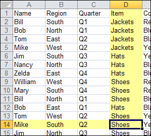
Figure 14.7. Use conditional formatting to highlight the selected cell in a table.
Caution
Do not use this method if you already have conditional formats on the worksheet. Any existing conditional formats will be overwritten. In addition, this program clears the Clipboard. Therefore, it is not possible to use this method while doing copy, cut, or paste.
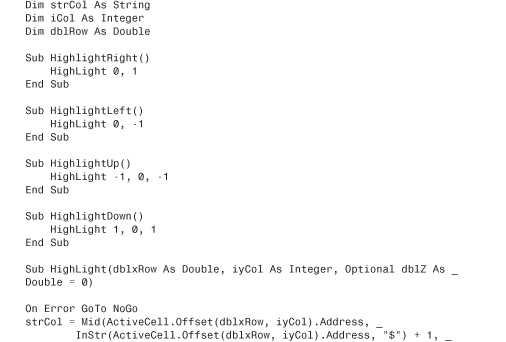
Highlight Selected Cell Without Using Conditional Formatting
Submitted by Ivan F. Moala.
This example visually highlights the active cell without using conditional formatting when the keyboard arrow keys are used to move around the sheet.
Place the following in a standard module:

Place the following in the ThisWorkbook module:

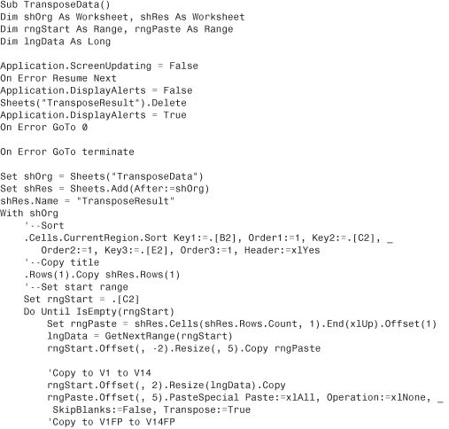
Custom Transpose Data
Submitted by Masaru Kaji.
You have a report where the data is set up in rows (see Figure 14.8). However, you need the data formatted so each date and batch is in a single row, with the Value and Finish Position going across. Note that the Finish Position is not shown in Figure 14.9. The following program does a customized data transposition based on the specified column, as shown in Figure 14.9.

Figure 14.8. The original data has similar records in separate rows.

Figure 14.9. The formatted data transposes the data so that identical dates and batches are merged into a single row.

Select/Deselect Noncontiguous Cells
Submitted by Tom Urtis.
Ordinarily, to deselect a single cell or range on a sheet, you must click an unselected cell to deselect all cells and then start over by reselecting all the correct cells. This is inconvenient if you need to reselect a lot of noncontiguous cells.
This sample adds two new options to the contextual menu of a selection: Deselect ActiveCell and Deselect ActiveArea. With the noncontiguous cells selected, hold down the Ctrl key, click the cell you want to deselect to make it active, release the Ctrl key, and then right-click the cell you want to deselect. The contextual menu shown in Figure 14.10 appears. Click the menu item that deselects either that one active cell or the contiguously selected area of which it is a part.
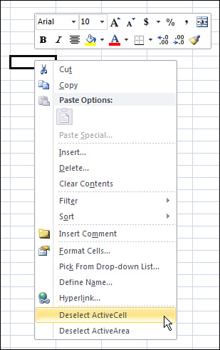
Figure 14.10. The ModifyRightClick procedure provides a custom contextual menu for deselecting noncontiguous cells.
Enter the following procedures in a standard module:
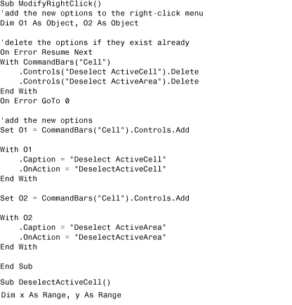
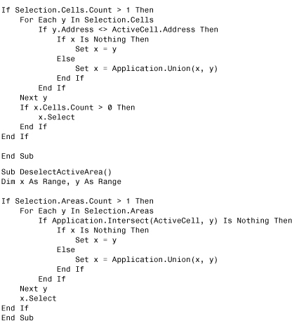
Add the following procedures to the ThisWorkbook module:

Techniques for VBA Pros
The next 10 utilities amaze me. In the various message board communities on the Internet, VBA programmers are constantly coming up with new ways to do something faster or better. When someone posts some new code that obviously runs circles around the prior generally accepted best code, everyone benefits.
Pivot Table Drill-Down
Submitted by Tom Urtis.
When you are double-clicking the data section, a pivot table’s default behavior is to insert a new worksheet and display that drill-down information on the new sheet. The following example serves as an option for convenience, to keep the drilled-down recordsets on the same sheet as the pivot table (see Figure 14.11) and letting you delete them as you want.
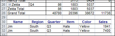
Figure 14.11. Show the drill-down recordset on the same sheet as the pivot table.
To use this macro, double-click the data section or the Totals section to create stacked drill-down recordsets in the next available row of this sheet. To delete any drill-down recordsets you have created, double-click anywhere in their respective current region.

Speedy Page Setup
Submitted by Juan Pablo Gonzàlez Ruiz of Bogotà, Colombia. Juan Pablo is an Excel consultant and runs his photography business at http://www.juanpg.com.
The following examples compare the runtimes of variations on changing the margins from the defaults to 1.5 inches and the footer/header to 1 inch in the Page Setup. The macro recorder was used to create Macro1. Macros 2, 3, and 4 show how the recorded code’s runtime can be decreased. Figure 14.12 shows the results of the speed test running each variation.

Figure 14.12. Page setup speed tests.


The macro recorder is doing a lot of extra work, which requires extra processing time. Considering this, along with the fact that the PageSetup object is one of the slowest objects to update, you can have quite a mess. So, a cleaner version that uses just the Delete key to clean out extraneous lines follows:

Okay, this runs faster than Macro1. The average reduction is around 70 percent on some simple tests! However, it can be improved even further.
As noted earlier, the PageSetup object takes a long time to process. Therefore, if you reduce the number of operations that VBA has to make and include some IF functions to update only the properties that require changing, you can get better results.
In the following case, the Application.InchesToPoints function was hard-coded to the inches value. The third version of Macro1 looks like this:
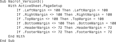
You will see the difference on this third version when you are not changing all the default margins.
Another option can reduce the runtime by more than 95 percent. This option uses the PAGE.SETUP XLM method. The necessary parameters are left, right, top, bot, head_margin, and foot_margin. These parameters are measured in inches, not points. Therefore, using the same margins that we have been changing already, a fourth version of Macro1 looks like this:
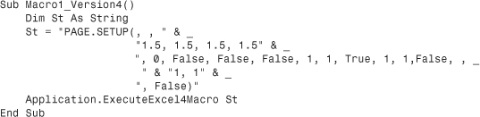
Caution
The second and fourth lines of St correspond to these parameters. However, you need to follow some simple precautions. First, this macro relies on XLM language, which is still included in Excel for backward compatibility. However, we do not know when Microsoft will drop it. Second, be care-ful when setting the parameters of PAGE.SETUP because if one of them is wrong, the PAGE.SETUP is not executed and does not generate an error, which can possibly leave you with the wrong page setup.
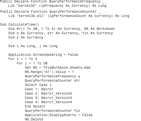
Calculating Time to Execute Code
You might wonder how to calculate elapsed time down to the thousandth of a second, as shown earlier in Figure 14.12.
This is the code used to generate the time results for the macros in this section:

Custom Sort Order
Submitted by Wei Jiang of Wuhan City, China. Jiang is a consultant for MrExcel.com.
By default, Excel enables you to sort lists numerically or alphabetically, but sometimes that is not what is needed. For example, a client might need each day’s sales data sorted by the default division order of belts, handbags, watches, wallets, and everything else. This sample uses a custom sort order list to sort a range of data into default division order and then deletes the custom sort order. Figure 14.13 shows the results.

Figure 14.13. When you use the macro, the list in A:C is sorted first by date, then by the custom sort list in Column I.

Cell Progress Indicator
Submitted by Tom Urtis.
I have to admit, the new conditional formatting options in Excel such as data bars are fantastic. However, there still isn’t an option for a visual like that shown in Figure 14.14. The following example builds a progress indicator in Column C based on entries in Columns A and B.

Figure 14.14. Use indicators in cells to show progress.


Protected Password Box
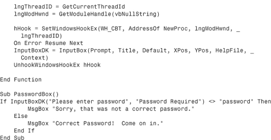
Submitted by Daniel Klann of Sydney, Australia. Daniel works mainly with VBA in Excel and Access, but dabbles in all sorts of languages.
Using an input box for password protection has a major security flaw: The characters being entered are easily viewable. This program changes the characters to asterisks as they are entered—just like a real password field (see Figure 14.15).

Figure 14.15. Use an input box as a secure password field.


Change Case
Word can change the case of selected text, but that capability is notably lacking in Excel. This program enables the Excel user to change the case of text in any selected range, as shown in Figure 14.16.

Figure 14.16. You can now change the case of words, just like in Word.


Selecting with SpecialCells
Submitted by Ivan F. Moala.
Typically, when you want to find certain values, text, or formulas in a range, the range is selected and each cell is tested. The following example shows how SpecialCells can be used to select only the desired cells. Having fewer cells to check will speed up your code.
The following code ran in the blink of an eye on my machine. However, the version that checked each cell in the range (A1:Z20000) took 14 seconds—an eternity in the automation world!

ActiveX Right-Click Menu
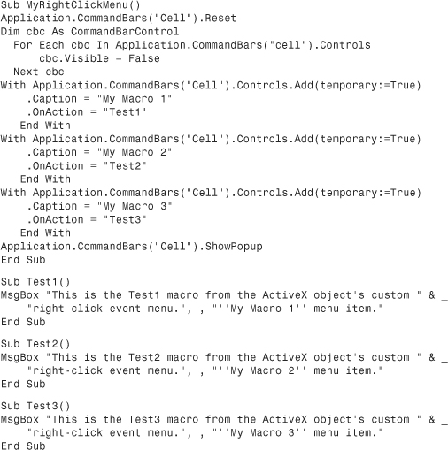
Submitted by Tom Urtis.
There is no built-in menu for the right-click event of ActiveX objects on a sheet. This is a utility for that, using a command button for the example in Figure 14.17. Set the Take Focus on Click property of the command button to False.

Figure 14.17. Customize the contextual (right-click) menu of an ActiveX control.
Place the following in the ThisWorkbook module:

Place the following in a standard module:
Cool Applications
These last samples are interesting applications that you might be able to incorporate into your own projects.
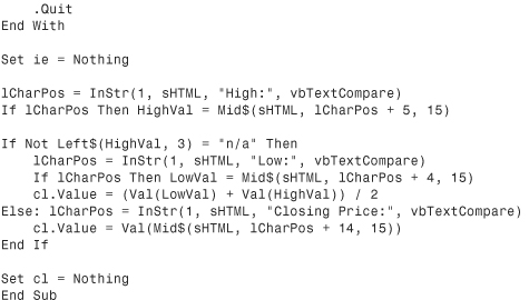
Historical Stock/Fund Quotes
Submitted by Nathan P. Oliver.
The following code retrieves the average of a valid stock ticker or the close of a fund for the specified date (see Figure 14.18).

Figure 14.18. Retrieve stock information.

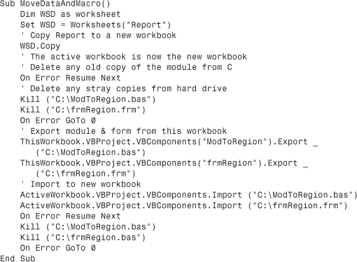
Using VBA Extensibility to Add Code to New Workbooks
You have a macro that moves data to a new workbook for the regional managers. What if you need to also copy macros to the new workbook? You can use Visual Basic for Application Extensibility to import modules to a workbook or to actually write lines of code to the workbook.
To use any of these examples, you must first open VB Editor, select References from the Tools menu, and select the reference for Microsoft Visual Basic for Applications Extensibility 5.3. You must also trust access to VBA by going to the Developer tab, choosing Macro Security, and checking Trust Access to the VBA Project Object Model.
The easiest way to use VBA Extensibility is to export a complete module or userform from the current project and import it to the new workbook. Perhaps you have an application with thousands of lines of code. You want to create a new workbook with data for the regional manager and give her three macros to enable custom formatting and printing. Place all of these macros in a module called modToRegion. Macros in this module also call the frmRegion userform. The following code transfers this code from the current workbook to the new workbook:
The preceding method will work if you need to move modules or userforms to a new workbook. However, what if you need to write some code to the Workbook_Open macro in the ThisWorkbook module? There are two tools to use. The Lines method allows you to return a particular set of code lines from a given module. The InsertLines method allows you to insert code lines to a new module.
Caution
With each call to InsertLines, you must insert a complete macro. Excel will attempt to compile the code after each call to InsertLines. If you insert lines that do not completely compile, Excel may crash with a general protection fault (GPF).

Next Steps
Excel 2007 and Excel 2010 offer fantastic new data-visualization tools, including data bars, color scales, icon sets, and improved conditional formatting rules. In Chapter 15, “Data Visualizations and Conditional Formatting,” you will learn how to automate the new tools and use VBA to invoke choices not available in the Excel user interface.