
2
Waves in Fluids
2.1 Introduction
The acoustic wave motion is described by the equations of aerodynamics that are linearized because of the small fluctuations that occur in acoustic waves compared to the static state variables. The fluid motion is described generally by three equations:
- Continuity equation – conservation of mass
- Newton’s law – conservation of momentum
- State law – pressure volume relationship.
For lumped systems the velocity is simply the time derivative of the point mass position in space. The same approach can be used in fluid dynamics, but here the continuous fluid is subdivided into several cells and their movement is described by trajectories. This is called the Lagrange description of fluid dynamics. Even if the equation of motions are simpler in that formulation it is quite complicated to follow all coordinates of fluid volumes in a complex flow. Thus, the Euler description of fluid dynamics is used. In this description the conservation equations are performed for a control volume that is fixed in space and the flow passes through this volume.
In this chapter, the three dimensional space is given by the Cartesian coordinates and the velocity of the fluid .
2.2 Wave Equation for Fluids
2.2.1 Conservation of Mass
For simplicity we consider first the flow in the -direction as in Figure 2.1. The mass flow balance contains the following quantities:
- The elemental mass with .
- Mass flow into the volume .
- Mass flow out of the volume .
- Mass input from external sources .

Figure 2.1 Mass flow in -direction through control volume.
Source: Alexander Peiffer.
leading to equation
for mass conservation. Expanding the second term on the right hand side in a Taylor series gives
and finally
This one dimensional equation of mass conservation in -direction can be extended to three dimensions:
The second term of (2.3) may be confusing, but it says that the change of density is not only determined by a gradient in the velocity field but also by a gradient of the density.
2.2.2 Newton’s law – Conservation of Momentum
The same procedure is applied to the momentum of the fluid. As shown in Figure 2.2 we get for flow in -direction:
- The momentum of the control volume is .
- The momentum flow into the volume .
- mass flow out of the volume .
- The force at position is .
- The force at position is .
- External volume force density .

Figure 2.2 Momentum flow in -direction through control volume.
Source: Alexander Peiffer.
Thus, the conservation of momentum in reads
Using Taylor expansions for and gives
Here, is the volume force density (force per volume). Using the chain law the partial derivatives of the first and second term lead to
The term in brackets is the homogeneous continuity Equation (2.1), and Equation (2.6) simplifies to
As with the conservation of mass, this can be extended to three dimensions:
This equation is the non-linear, inviscid momentum equation called the Euler equation.
2.2.3 Equation of State
The above equations relate pressure, velocity and density. For further reducing this set we need a third equation. The easiest way would be to introduce the . Here we start with the first law of thermodynamics in order to show the difference between isotropic (or adiabatic) equation of state and other relationships.
With the following specific quantities per unit mass
 (2.10)
With the specific entropy we get:
 (2.10)
The relation comes from the fact that is a mass specific value and therefore the reciprocal of the density . For an ideal gas we have
and are the specific thermal heat capacities for constant pressure and volume, respectively. That is the ratio of temperature change per increase of heat . From the total differential
we can derive
Using all above relations the change in density is:
with . In most acoustic cases the process is isotropic: i.e. time scales are too short for heat exchange in a free gas; thus , and the change of pressure per density is
In case of constant temperature (isothermal) we get with (2.12) and the ideal gas law (2.11):
As we will later see, is the . Newton calculated the wrong speed of sound based on the assumption of constant temperature that was later corrected by Laplace by the conclusion that the process is adiabatic. For fluids and liquids like water a different quantity is used because there is no such expression as the ideal gas law. The bulk modulus is defined as:
Due to (2.15) and (2.16) the relationship between the bulk modulus and is:
The bulk modulus can be defined for gases too, but we must distinguish between isothermal or adiabatic processes.
2.2.4 Linearized Equations
Equations (2.3) and (2.8) can be linearized if small changes around a certain equilibrium are considered:
Inserting (2.22) into the equation of continuity (2.3), neglecting all second order terms as far as source terms, and setting1 the linear equation of continuity is:
Doing the same for the equation of motion (2.8) leads to:
Using the curl of this equation it can be shown that the acoustic velocity can be expressed using a so-called velocity potential which will be useful for the calculation of some wave propagation phenomena.
2.2.5 Acoustic Wave Equation
From the following operation
follows
With the equation of state (2.15) for the density we get the linear wave equation for the acoustic pressure
Inserting the velocity derived from the potential into the linear equation of motion (2.24) provides the required relation between pressure and the velocity potential
Thus, the relationship between pressure and the velocity potential is
Entering this into the wave equation (2.27) and eliminating one time derivative gives:
The definition of the velocity potential (2.25) and equation (2.29) can be applied for the derivation of a relationship between acoustic velocity and pressure:
2.3 Solutions of the Wave Equation
In acoustics we stay in most cases in the linear domain, so we change the notations from equations (2.20)–(2.22):
Equations (2.27) and (2.30) define the mathematical law for the propagation of waves. For the explanation of basic concepts the wave equation is used in one dimensional form.
2.3.1 Harmonic Waves
According to D’Alambert every function of the form is a solution of the one-dimensional wave equation. In the following we will consider harmonic motion or waves so we replace the functions and by the exponential function with
and get
The first term of the right hand side of this equation is travelling in positive directions, the second in negative directions2. Harmonic waves are characterized by two quantities, the angular frequency and the wavenumber . The first is the frequency (in time) as for the harmonic oscillator, and the second is a frequency in space. A similar relationship can be found between the time period and the wavelength . Space and time domains are coupled by the sound velocity as shown in Table 2.1.
Table 2.1 Quantities of wave propagation in time and space domains.
| Name | Time | Space | ||
|---|---|---|---|---|
| Symbol | Unit | Symbol | Unit | |
| Period | s | m | ||
| Frequency | s(Hz) | m | ||
| Angular frequency | s | m | ||
The time integration in Equation (2.31) corresponds to the factor and reads in the frequency domain:
For one-dimensional waves in the -direction this leads to:
Depending on the wave orientation the ratio between pressure and velocity is given by:
In accordance with the impedance concept from section 1.2.3 we define the ratio of complex pressure and velocity as specific acoustic impedance
also called acoustic impedance. For plane waves this leads to:

Figure 2.3 One-dimensional harmonic waves travelling in the positive -direction (m/s, s).
Source: Alexander Peiffer.
is called the characteristic acoustic impedance of the fluid. The specific acoustic impedance is complex, because for waves that are not plane the velocity may be out of phase with the pressure. However, for plane waves the specific acoustic impedance is real and an important fluid property.
The above description of plane waves can be extended to three-dimensional space by introducing a wavenumber vector .
2.3.2 Helmholtz equation
Entering (2.40) into the wave Equation (2.27) provides
The term is often omitted and with we get the homogeneous.
2.3.3 Field Quantities: Sound Intensity, Energy Density and Sound Power
A sound wave carries a certain amount of energy that is moving with the speed of sound. We start with the instantaneous acoustic power :
is the force acting on a fluid particle and the associated velocity. The acoustic intensity is defined as the power per unit area in the direction of the unit vector and with we get:
As in Equation (1.48) the time average is given by:
Using the harmonic plane wave solutions for pressure (2.34) and velocity (2.36)

the time averaged mean intensity yields:
and finally:
We see that the specific impedance relates the intensity to the squared pressure.
The kinetic energy density in a control volume is written as
The potential energy density follows from the adiabatic work integral as in equation (2.9)
If we use Equation (2.15) we get the change in density as a start for the change in volume
With unit mass in the control volume it follows from that
Finally we get:
Pressure and velocity are in phase for plane waves; the same is true for the potential and kinetic energy density, so the total energy density is given by:
Using Equation (2.34) the time average over one period leads to:
Finally, we can see that the speed of sound relates energy density to the sound intensity.
All those above expressions are useful for the description and evaluation of sound fields. Especially in case of statistical methods that are based on the energy density of acoustic subsystems they link the wave fields to the energy in the systems and the power irradiating at the system boundaries.
If the intensity can be determined over a certain surface the source power is calculated by integrating the intensity component perpendicular to the surface
2.3.4 Damping in Waves
There is no motion without damping, and a sound wave propagating over a long distance will vanish. This is considered by adding a damping component to the one-dimensional solution of the wave equation similar to the decay rate in (1.22)
Here is the damping constant. There are several reasons for the attenuation of acoustic waves:
- Viscous damping due to inner viscosity.
- Thermal damping due to irreversible heat flow during wave propagation.
- Molecular damping due to excitation of degrees of freedom of molecules (for additional content of the gas, e.g. humidity in air).
The damping loss as defined in (1.68) is based on the amount of energy dissipated during one cycle of wave motion. The harmonic pressure wave performs one cycle of oscillation in one period in time or space . So we get for :
For small damping the exponential function can be approximated by providing the relationship between damping loss and fluid wave attenuation.
Hence, the attenuation can be given by:
An appropriate way to consider this relationship in the solution of the wave equation is to include this into a complex wavenumber :
This complex wavenumber naturally impacts the speed of sound
and the acoustic impedance
The shown quantities of the plane wave field can also be applied in three-dimensional space and they are summarized in Table 2.2.
2.4 Fundamental Acoustic Sources
The radiation of sound is key to understanding how energy is introduced into wave fields. Depending on the wavelength, geometry, and dimension of the source the behavior varies. A detailed understanding of fundamental sources is helpful for the radiation of vibrating structures and thus, how they exchange acoustic energy.
2.4.1 Monopoles – Spherical Sources
The most simple geometry we might think of is a point in space. For simple derivation of the sound field of a point source the spherical coordinate system is introduced as shown in Figure 2.4 and defined by the following coordinate transformation

Figure 2.4 Definition of a spherical coordinate system.
Source: Alexander Peiffer.
Using this coordinate system and neglecting the angular components the Laplace operator reads as
The wave equation for the velocity potential (2.30) becomes
The two right terms can be written in a different form using as argument
Equation (2.30) is the one-dimensional wave equation for the argument , so we can use the D’Alambert solution

Figure 2.5 Breathing sphere as source model for a monopole.
Source: Alexander Peiffer.
The first term represents an outgoing wave travelling away from the source, the second an incoming wave travelling to the source. As we are interested in sound being emitted from the source we consider the outgoing harmonic solution with complex amplitude
Consider a pulsating sphere of radius in the centre with normal surface velocity . With the velocity potential the radial velocity can be easily derived from the solution (2.67):
Substituting Equation (2.67) into (2.68) and solving for gives
Hence,
The strength of the source is defined by the volume flow rate. This is the surface of the sphere times normal velocity
With the harmonic source strength
the spherical wave solution is
Using equations (2.25) and (2.35) pressure and velocity are given by
and
2.4.1.1 Field Properties of Spherical Waves
The acoustic impedance is according to Equation (2.38)
In contrast to the plane wave, the specific acoustic impedance is not real. It contains a resistive and a reactive part. When the resistive part is dominant the pressure is in phase with the velocity. When the reactive part dominates, the velocity is out of phase to the pressure. The out of phase component does not generate any power in the sound field as it was the case for moving a mass or driving a spring. The motion is partly introduced into the local kinetic energy, and this part can be recovered as it is the case for an oscillating mass. For the acoustic field of a spherical source the reactive field represents the near-field fluid volume that is carried by the sphere motion but not emitting a wave.

Figure 2.6 Reactance and resistance of specific acoustic impedance of a pulsating sphere.
Source: Alexander Peiffer.
There are two limit cases in Equation (2.76):
- ; the wave length is much larger than distance .
- ; the wave length is much smaller than distance .
Introducing the above approximations into Equation (2.76) gives a fully reactive impedance for (i)
and a resistive part equal to plane waves for (ii)
2.4.1.2 Field Intensity, Power and Source Strength
The time averaged radiated intensity is
The total radiated power can now be evaluated from Equation (2.54) and the integration surface
The mean square pressure can be derived from (2.74) and expressed by the intensity using (2.45)
Replacing the intensity in (2.81) gives the rms pressure in the spherical sound field due to power
2.4.1.3 Power and Radiation Impedance at the Surface Sphere
The characteristic impedance of the sphere exactly at the surface at radius can be translated into the radiation impedance of the sphere as a volume source. The radiation impedance is defined as the ratio of pressure to source strength at the vibrating surface
If we assume a constant harmonic surface velocity we get for the radiation impedance of the breathing sphere and according to the acoustic impedance (2.76)
The acoustic radiation impedance is the ratio pressure and normal velocity at the sphere’s surface
We can now use this impedance to eliminate either or . The power transmitted by a vibrating sphere using Equation (2.54) over the surface of the sphere
or for constant source pressure
It is instructive to see the mechanical properties considering the limit cases from above and extract the mass that is moved by the surface. From Newtons’s law a force given by leads to an in-phase acceleration of of a mass
hence
For we get: . Thus, at low frequencies the source surface motion carries three times the fluid volume of the sphere. This motion near the source is called an evanescent wave, because it is oscillatory motion of fluid that does not radiate.
2.4.1.4 Point Sources
A point source is a spherical source with an infinitely small radius. Performing the limit for Equation (2.73) leads to the velocity potential for point sources of strength
The pressure and velocity field of such a source is given by
and
All other relations regarding power and intensity expressions remain. We see that the limit is expressed for and not for the wavelength. The reason is that it is the ratio of a characteristic length (in this case the sphere radius) to the wavelength that determines if the geometrical details must be considered or not. In other words, a wave of a certain wavelength doesn’t care about details that are much smaller.
With the D’Alambert solution for spherical waves (2.66) we can also derive a point source in time domain
The point source is of great importance for the solution of the inhomogeneous wave equation in combination with complex boundary conditions. Any source can be reconstructed by a superposition of point sources as shown in Section 2.7.
Performing the limit process with and taking the power from equation 2.86 we get the intensity of the point source:
and the total radiated power
with radiation impedance following from this
2.5 Reflection of Plane Waves
A plane wave striking a plane surface is a first example of interaction with obstacles. Imagine a configuration as shown in Figure 2.7. The impedance of the surface is , and it is given by using the velocity perpendicular to the plane.

Figure 2.7 Reflection of a plane wave at an infinite surface with impedance .
Source: Alexander Peiffer.
Without loss of generality the wave front is parallel to the -axis and all properties are functions of and . The solution in the half space of is the superposition of two plane waves.
With the following arguments of the exponential function
The pressure at the surface is given by
and the velocity in -direction reads
 (2.101)
We certainly shall not be able to match the impedance at every surface position unless the arguments of the exponential functions are equal, hence
So, we get from the surface impedance condition
With and rearranging the above equation, the reflection factor is given by
The ratio between irradiated power to reflector power is the squared reflection factor called the.
Note that those coefficients are exclusively described by the impedance of fluid and surface and not density or speed of sound. Thus, the impedance is the relevant quantity here.
2.6 Reflection and Transmission of Plane Waves
A plane wave passing a flat interface between two infinite fluid volumes with different density and sound velocity as shown in Figure 2.8 is a first example of continuous systems exchanging acoustic energy. Applications of such a system could be for example the interface between a liquid (water) and a gas (air) or just different gases.

Figure 2.8 Transmission and reflection of a plane wave at the interface of two fluids.
Source: Alexander Peiffer.
Region 1 of the incoming wave has two wave components, the incoming and the reflected wave, and region 2 the transmitted wave. Thus, both velocity potentials read
Using the given angles as sketched in Figure 2.8 the wavenumber space vector products are given by
with and . The contact face between the fluid requires the continuity of pressure and velocity in the -direction. We start with the pressure . Entering equations (2.107)–(2.109) into (2.106) and determining the pressure relation
gives
A solution for any is only possible if the arguments of the exponential functions are equal.
So also in the transmission case the incident angle equals the angle of the reflected wave. Additionally we have
This represents the acoustic equivalent of Snell’s law of transmission:
With these conditions we can factor out the exponential function
After clarifying the angles of reflection and transmission the next point is to assess the fraction of transmitted and reflected wave. From the continuity condition for the velocity in the -direction we get with when going through the algebra
Rearranging equations (2.114) and (2.115) the reflection factor is
 (2.116)
This expression is similar to (2.103) except the angle factor that represents the physics of the wave propagation in the second medium. The transmission factor is defined by the ratio of pressure amplitudes and . Hence,
 (2.117)
The transmitted acoustic power follows from the square of the amplitudes. We introduce a transmission coefficient by
Without loss of generality we assume so each power is given by
With (2.117) this reads as:
It should be noted that the transmission coefficient of the flat interface between two fluids is determined by the impedance of each half space ‘seen’ from the other side. This is the first indication for the coupling of subsystems determined by the radiation impedance into the free fields of each subsystem. Similar expressions will be found in Sec. 8.2.4.1 when transmission is dealt with in the context of coupled random subsystems.
2.7 Inhomogeneous Wave Equation
In the considerations in this chapter so far, we neglected the source terms related to the conservation of mass and momentum. All sources discussed until now are caused by vibrating surfaces. For establishing a physical link between the source term and the specific mass flow in Equation (2.3) and force density term in Equation (2.8) we keep the terms this time. The source terms are not influenced by the linearization procedure; thus, the inhomogeneous and linear equations of momentum (2.24) and continuity (2.23) read as
Repeating the steps of section 2.2.5 we finally get the inhomogeneous wave equation
The density source is converted into a volume source strength density by . The above equation can also be converted into the frequency domain and hence to the inhomogeneous Helmholtz equation
2.7.1 Acoustic Green’s Functions
This section presents the concept of the Green’s function that uses a formalism to calculate the sound field for arbitrary source and boundary configurations as shown for example by Morse and Ingard (1968).
The Green’s function is defined as the solution of the following inhomogeneous wave equation.
The inhomogeneous part is the delta function which allows for this elegant derivation of the Kirchhoff integral. The delta function is introduced in the appendix A.1.3 in the time domain. However, it can also be applied in space. The multidimensional delta function is simply the product of three Dirac delta functions in space
The sifting properties and the value of the integration is defined by volume integral
The solution of Equation (2.124) is the point source (2.91)3.
In order to achieve a common formulation we add an arbitrary solution of the homogeneous wave equation
to the Green’s function to get the generalized Green’s function
The purpose of the additional homogeneous solution is to create freedom to fulfill boundary conditions that do not occur in the free sound field. The task is to find the solution for the inhomogeneous wave equation
The generalized Green’s function must be a solution of the following equation for the special case with and the boundary as shown in Figure 2.9.

Figure 2.9 Solution volume and boundaries.
Source: Alexander Peiffer.
In order to receive a global solution we perform the operation
This leads to
Exchanging and and integrating over the volume gives
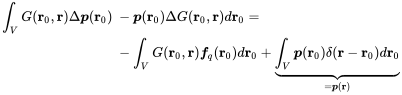 (2.134)
The last term on the RHS follows from the sifting property of the delta function
 (2.135)
With Green’s law of vector analysis
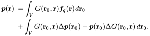
some volume integrals can be transferred into surface integrals and we get finally
 (2.137)
The first term on the right-hand side is the volume integral over all sources in the volume. So given a known source distribution we can calculate the according sound field. The two terms in the surface integral take care of the boundary condition. The pressure gradient in the first can be converted into the normal velocity using (2.35). The second surface integral allows establishing the correct surface impedance. Equation (2.137) is called the constant frequency version of the .
2.7.2 Rayleigh integral
The Rayleigh integral is a special solution of the Kirchhoff-Helmholtz integral applied to flat and infinite surfaces. We assume a configuration as shown in Figure 2.10. The integration volume is the right half space for closed by a half sphere of infinite radius. The Green’s function of any source at with is as defined in equation (2.127). The rigid surface acts as a reflector. Thus, there is a mirror source located at . This source is not in volume , and the added wave field is therefore considered as a homogeneous solution in the volume. Hence, we get for the generalized Green’s function

Figure 2.10 Half space in front of a rigid wall.
Source: Alexander Peiffer.
We enter this version of the Green’s function in Equation (2.137) and we get
 (2.139)
We assume a source-free half space so , and due to the mirror source symmetry is also true. By clever selection of the Green’s function we fulfilled the boundary condition automatically. For the surface integral the contributions from the half sphere with infinite radius are supposed to be zero. From Equation (2.35) the first expression can be converted into an expression for the surface velocity . Performing the limit process we get
and with this Green’s function we can derive the Rayleigh integral that allows the calculation of infinite half space sound fields excited by a rigid vibrating plane with arbitrary velocity distribution .
2.7.3 Piston in a Wall
A cylindrical loudspeaker in a wall can be modelled by a piston of radius vibrating with velocity located in a rigid wall. For convenience the surface integral will be expressed in cylindrical coordinates and . The receiver coordinates are given as spherical coordinates and (Figure 2.11). Without loss of generality the azimuthal angle is set to zero.
 (2.142)
Figure 2.11 Coordinate definitions for the piston in the wall.
Source: Alexander Peiffer.
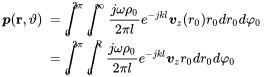
In the far field approximation we assume and get
So, the approximate result is
The integral is the Bessel function of first order
The results for some values of are shown in Figure 2.12 over the angular range of . For a piston size small compared to the wavelength () the radiation pattern is similar to a point source. The smaller the wavelength gets in relation to the piston radius the more a specific radiation pattern develops.

Figure 2.12 Angular distribution (radiation pattern) of the pressure field of the piston.
Source: Alexander Peiffer.
2.7.3.1 Impedance Concept
The radiation impedance of the piston is calculated from the pressure averaged over the surface related to the piston velocity . As shown by Lerch and Landes (2012) the mechanical impedance of the piston due to radiation is given by
According to equation (2.141) assuming a constant velocity over the surface the pressure is
Thus, we get the pressure at from integrating the contribution from the rest of the piston in circles of radius . The angle integration over runs from to . From every angle follows the integration limits of the second integral.
Using those limits gives
 (2.149)
Inserting equation (2.149) into (2.146) leads to the expression

Figure 2.13 Surface integration over piston for radiation impedance.
Source: Alexander Peiffer.
Running through quite a lot of algebraic modifications we get the expression for the impedance of a piston
or
is the Hankel function of first order. In Figure 2.14 the real and imaginary parts of the acoustic radiation impedance are compared to those of the pulsating sphere. Both sources have a similar shape except some waviness for the piston resulting from interference effects from the integration over the piston surface. For large the impedance is real for both radiators and approaches the acoustic impedance of a plane wave .

Figure 2.14 Acoustic radiation impedance of the piston.
Source: Alexander Peiffer.
With Equation (2.87) the radiated power of a piston of source strength is
The main use of Equation (2.153) is that the required velocity to achieve (or prevent) a certain sound power can be calculated from it, for example if one must define the boundary condition for a radiating piston in simulation software and only the radiated power is known.
2.7.3.2 Inertia Effects
The Bessel functions can be approximated by a series in taking the first series term of both functions (Jacobsen, 2011)
This expression is valid for . From the imaginary part we get for the mass
Assuming a cylindrical volume of the fluid above the piston we can calculate the length of the moving mass cylinder to be
meaning that at low frequencies the piston is moving a fluid layer of times the radius acting as an inertia without radiation.
2.7.4 Power Radiation
For the radiated power calculation of the piston we took the pressure at the piston surface and integrated the pressure–velocity product over the surface. Due to the fact that the velocity is constant the surface integral involves mainly the pressure as a space-dependent property. In case of vibrating structures with complex shapes of vibration the velocity distribution over the surface is not homogeneous, and we need a more detailed approach.
 (2.157)
In the above equation a function with argument is multiplied by the velocity function for and integrated over the two-dimensional space. Mathematically, this can be interpreted as a two-dimensional convolution in space
Thus, when we apply the two-dimensional Fourier transform to the Rayleigh integral the result is the product of the Fourier transform of the vibration shape and the Green’s function in wavenumber space leading to
So, we have replaced the expensive convolution operation by a multiplication. This simplification is at the cost of two-dimensional Fourier transforms that are required to get the expressions in wavenumber domain.
The time averaged intensity of a sound field is given by the product of pressure and velocity (2.45). As the velocity is not uniform over the surface we perform a surface integration over the vibrating area to get the total radiated power
 (2.160)
Thus, for the determination of radiated power a double area integral is required that may become computationally expensive.
In the above expression we can also switch to the wavenumber domain. In this case the area integration is replaced by an integration over the two-dimensional wavenumber space.
 (2.161)
The double integral is replaced by a single two-dimensional wavenumber integration. Thus, once the shape function is available the power calculation in wavenumber space is much faster than in real space (Graham, 1996).
2.7.4.1 Radiation Efficiency
The radiation efficiency is a quantity that relates the power of a plane wave to the radiated power of a vibrating surface with same surface averaged velocity. The definition of the radiation efficiency was motivated by experimental procedures because it allows the estimation of the radiated power from the measurements of the vibration velocity. The squared average velocity of a vibrating surface is
and the power radiated by a plane wave through the same area is given by (2.47)
The radiation efficiency is defined as the ratio between the radiated power of a velocity profile of a surface and the standardized power of the plane wave:
The radiation efficiency is used to determine the radiated power of vibrating structures from calculated, estimated, or measured radiation efficiency of specific surfaces
2.8 Units, Measures, and levels
The dynamic range of acoustic quantities can be very high; thus, a logarithmic scale is well established for the quantification of acoustic signals. For convenience a certain time averaged quantity, for example the mean square pressure , is compared to a mean square reference value . The pressure level in decibels is defined as follows:
The factor of 10 is introduced to spread the scale. Linear quantities such as pressure, velocity, or displacement use the mean square values. As level and decibel are used on time signals too, one should not apply the decibel scale to amplitudes. This may lead to confusion, as it is not clear if the mean square values of the amplitude is meant. This makes even more sense when the energy and power levels are defined. The energy must be averaged, as there is no constant value over the period – see Equation (2.46). Energy quantities such as energy, intensity, or power are compared with mean values and not mean square values; hence:
Table 2.3 Field and energy properties of acoustic waves
| Source | Source strength | Impedance Velocity | Pressure Radiated power |
|---|---|---|---|
| Mono pole | |||
| Breath. sphere | |||
| Piston | |||
In addition, the decibel scale is used for ratios of similar quantities. A typical example is the transmission loss that is the decibel scale of the transmission factor from Equation (2.118) that relates the transmitted to the radiated power. The definition of the transmission loss (TL) is:
The reciprocal definition was chosen in order to get positive values for losses. When linear quantities are compared, for example the pressure at two locations, the mean square values are related. When the squared pressure is compared to the situation with and without a specific equipment or installation, this is called insertion loss (IL)
The reference quantities for power and pressure are chosen conveniently to simplify the calculations with levels. Taking the equation for the spherical source (2.82) and dividing it by the squared reference value for the pressure yields
and taking the decibel of this
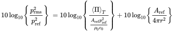
yields
Entering typical values for air with kg/m and m/s using m we get
matching well to the reference value of acoustic power.
Bibliography
- W.R. Graham. BOUNDARY LAYER INDUCED NOISE IN AIRCRAFT, PART I: THE FLAT PLATE MODEL. Journal of Sound and Vibration, 192(1): 101–120, April 1996. ISSN 0022-460X.
- Finn Jacobsen. PROPAGATION OF SOUND WAVES IN DUCTS. Technical Note 31260, Technical University of Denmark, Lynby, Denmark, September 2011.
- Reinhard Lerch and H. Landes. Grundlagen der Technischen Akustik, September 2012.
- P.M.C. Morse and K.U. Ingard Theoretical Acoustics. International Series in Pure and Applied Physics. Princeton University Press, 1968. ISBN 978-0-691-02401-1.
Notes
- 1 Keeping would lead to the convective wave equation that is used in the context of flow related acoustic problems, which is more a topic of aero acoustics
- 2 Negative means propagation in positive -direction, because of the convention. This is the reason why pure acoustic textbooks usually take the convention in order to get positive wavenumber for positive propagation.
- 3 This can be proven using the relationship between the and exponential functions