
Appendix B
Specific Solutions
B.1 Second Moments of Area
The bending wave behavior of beams is determined by the cross-section of the beam. We saw in Equations (3.94)–(3.95) that those quantities are a result of an area integration for the infinitesimally small area times the lever related to the neutral axis. There are some definitions and rules that are mandatory to deal with beam dynamics. Figure B.1 shows a typical cross section from building construction. The I or double T-beam. The second moments of area for the axis through the centroid and thus neutral axes are

Figure B.1 Cross section of I-beam with axes coinciding with the centroid. Source: Alexander Peiffer.
Here, the first two terms are called the second moment of area with respect to the and axes, respectively. The last term is called the product moment of area. There is a further moment linked to the torsion of the beam, the polar moment of area
The polar moment is related to the area moment by the perpendicular axis theorem:
If, for instance, a beam is made up of several standard sections or it is mounted on a plate that defines the neutral axis, the transformation to different axes is required. The moments of area regarding the axes and are:
In addition one might rotate the coordinate system around the center by leading to the new axes . The updated moments are
From Equation (B.11) it follows that you can always find an angle with
Those axes that fulfill this requirement are called the principle axes of the cross-section. For symmetric sections they coincide with the axes of symmetry.
B.2 Wave Transmission
In contrast to the hybrid coupling loss factor formulation from section 7.3 based on the diffuse field reciprocity, the wave based theory relies on the transmission and reflection of plane waves. This theory was derived by Langley and Heron (1990) for plate edges and from Langley and Shorter (2003) for point connections. For plane acoustic waves a similar approach was shown in section 2.6 for the introduction of the wave transmission coefficient. The coupling loss factor can equivalently be derived from the transmission coefficient. For one- and two-dimensional junctions, the diffuse field transmission must then be calculated by averaging over the appropriate angles.
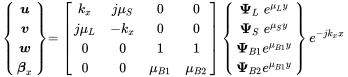
For plates we have four wave types, and the transmission and reflection is rather complex and must be expressed by several transmission coefficients. For arbitrary line junctions the extension to plane wave transmission based on the theory shown in section 8.2.5.1 is achieved by extending the solution of pure radiating waves in Equations (8.115)–(8.118) by selecting one specific incoming wave from
 (B.13)
For we get the edge formulation as in Equation (8.133). In short form the out-going wave field of (B.13) reads:
Applying the differential equations of the free edge (8.108a)–(8.108d) to the above solution of four radiating waves gives the equations of motion in wave amplitude coordinates as given by the block matrices from (8.120) and (8.123).
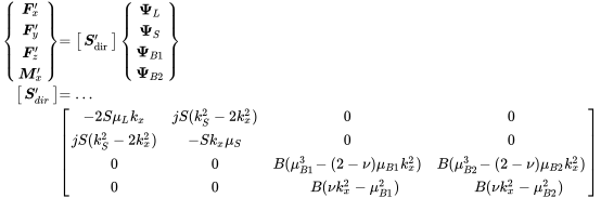 (B.15)
The inverse wave transformation matrix provides the radiation stiffness in edge coordinates
For plates with purely out-going waves, the above equation is valid. Imagine a plate that carries out-going waves and one incoming wave of the form:
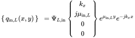 (B.17)
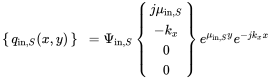 (B.18)
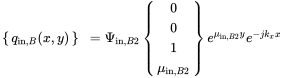 (B.19)
For the incoming waves the evanescent bending wave can be omitted because it cannot propagate. The incoming waves change in sign and are related to the outgoing by
The wave field on the plate carrying both waves, one incoming and all out-going waves, can be described by:
Applying boundary conditions (8.108a)–(8.108d) on the full wave field gives for the specific edge force
The edge motion is a combination of both waves. Hence,
and using this gives
When no external forces are acting on the edge we may rewrite
So, the right hand side of the above equation may be interpreted as the blocked force generated by the incoming wave
If we assume the th plate carrys the incoming wave, the global edge motion of the full junction follows from this force transformed into the global edge system
acting on the total stiffness of the full line junction (8.129)
The solution of (B.28) provides the edge motion in global coordinates. Rotating into the coordinate system of the th plate and applying the wave transformation matrix provides the amplitude of each wave:
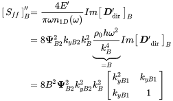
For the determination of the transmission coefficient we must calculate the radiated and irradiated power. Due to the infinite length of the line, this must be a length intensity. In addition, it is weighted by the angle to consider only the component orthogonal to the line edge.
With denoting the subsystem, the wave type . For example is the group velocity of the -wave of the th plate. The energy density follows from the area density and the displacement amplitudes with1
Note that due to the formulation of the in-plane wave propagation, is not the displacement amplitude in these cases. The amplitudes are , and for longitudinal, shear and bending waves, respectively.
Finally the intensities for each wave type are
The incoming wave and angle drives the wavenumber ; the transmitted angles follow from the transmitted wavenumbers
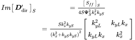
Finally the transmission coefficient follows from the ratio of transmitted to irradiated intensity
When there will be no solution for and . So, not all wave types are available for all angles. For example in Figure B.2 the full angle of the shear wave leads to a minimal angle that does not start at zero, because longitudinal waves occur first when the projected wavenumber is equal to or smaller than .

Figure B.2 Angle range for shear wave with given 0–90∘ range of longitudinal wave. Source: Alexander Peiffer.
The wave transmission theory has one advantage: it is also valid for strong coupling, for example a transmission factor of when similar plates are coupled together at an angle of 180∘. The diffuse field reciprocity requires a diffuse field, which is hard to achieve with fully coupled and therefore fully absorbing boundary conditions.
B.2.1 The Blocked Forces Interpretation
The following term was described in Section B.2 as the blocked force
It is worth illustrating this fact in more detail. The incoming wave generates the force given by the boundary conditions of the edge and an edge motion . In order to achieve the bocked boundary condition, a force must act in such a way on the boundary that it excites an out-going that matches exactly the incoming wave with negative sign, thus:
This force is given by
So in total, the edge must act with force in order to block the edge motion of an incoming wave. From the force balance follows that the incoming and reflected wave acts with the force as shown in Equation (B.26).

Figure B.3 In-coming and out-going waves assuring the blocked condition at boundary . Source: Alexander Peiffer.
There are further consequences. First, for the calculation of waves that are reflected in one sense but transmitted into a different wave type but the same plate, the reflected blocked force components must by subtracted. The easiest way to do so is to subtract from the global solution in Equation (B.28). Second, for the realization of the blocked force of one wave type, the in-plane wave requires both in-plane waves. Thus, there is an inert exchange of energy between both subystems that breaks the rule for the diffuse field reciprocity.
In the remainder of Section B.2, the blocked forces for each wave type are derived in detail. According to the diffuse field reciprocity (7.19), this blocked force is also given by the free field radiation stiffness of each wave type. This separation into waves is clear for bending waves, but not for the in-plane waves where the edge motion usually generates a combination of both wave types, shear and longitudinal waves.
B.2.2 Bending Waves
The wave solution for incoming bending waves relies on the positive and real wavenumber solution and . Using this and setting the evanescent wave , the incoming wave reads as
With we get the edge displacement:
and for the traction force vector
The reaction to the edge displacement follows from the radiation stiffness times the edge motion
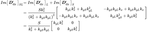
Using these equations in (B.36) gives the blocked reverberant force due to bending waves
For further consideration it is better to replace the propagation constants by wavenumber expressions
Using the this convention
leads to the cross spectral density matrix:
This cross spectrum is per square length, as the force is a specific force per length.
For the consideration of the reciprocity, the modal density of plates and expression for the total energy is required. As explained in section 8.2.4.1, the plane wave formulation with the projected wavenumber as degree of freedom has to be treated as a one-dimensional system.
From Figure B.4 it follows that the effective length follows from and the wavenumber ratio.

Figure B.4 Effective subsystem length for plane waves in two-dimensional systems.
Together with , we get the modal density
The energy in the plate subsystem is given by
In this case the energy length density is required, thus
For the determination of the radiation stiffness, the same convention of the propagation constants (B.45) is used
With the modified length specific diffuse field reciprocity (7.19) we get finally:

This proves the diffuse field reciprocity in case of bending waves of homogeneous plates.
B.2.3 Longitudinal Waves
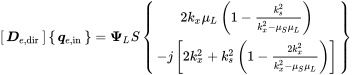
The wave solution for incoming longitudinal waves relies on the positive solution . Using this the incoming wave reads as:
with we get the edge displacement
and for the traction force vector
The reaction to the edge displacement follows from the radiation stiffness times the edge motion
 (B.58)
Using these equations in (B.36) gives the blocked force due to longitudinal waves
For further consideration the propagation constants are replaced by wavenumber expressions
Using this convention
leads to the cross spectral density matrix
With the effective length
and the fact that for and -waves, the group velocity equals the phase velocity , we get the modal density
The energy in the plate subsystem is given by
Note that the amplitude for in-plane waves is given as a product including the wavenumber. So, the longitudinal wave amplitude displacement is given by . The energy length density reads as
The diffuse field reciprocity requires the following expression to relate the radiation stiffness to the cross spectrum
In the above equation the mass per area can be replaced using the expression for the wavenumber (3.167)
With the identity we get
With the modified length specific diffuse field reciprocity (7.19) we get finally
 (B.68)
This matrix can be used as imaginary of the radiation stiffness, but this is not derived from diffuse field reciprocity. The radiation stiffness is defined by a coupled motion of both waves, making it impossible to identify a pure longitudinal wave radiation.
B.2.4 Shear Waves
Following the similar procedure as in section B.2.3 with an incoming shear wave, the blocked force reads
As illustrated in Figure B.2, there is an angle or wavenumber range where both propagation constants are complex, but also a range where is real and only remains imaginary. For we use (B.60)
giving the following blocked force matrix
Applying shear wave quantities to the one-dimensional modal density and energy gives
Using we get
 (B.73)
In the wavenumber range only remains real, and we keep the longitudinal propagation constant
The cross correlation provides
We note that the diffuse field reciprocity is impossible to fulfill here, because the matrix contains imaginary components. However, if we ignore this fact, and with the diffuse field reciprocity factor (B.72), we get
 (B.76)
B.2.5 In-plane Waves
Both waves can be combined by adding both radiation imaginary parts of the radiation stiffnesses (B.68) and (B.73)
 (B.77)
In contrast to this the imaginary of the in-plane stiffness matrix (8.121) reads
So, except the off diagonal components, the blocked force cross correlation is equal to the imaginary radiation stiffness. This equation is valid for ; for , Equation (B.76) must be used as there is no propagating longitudinal wave. For the comparison to the combined in-plane stiffness matrix (8.121), we use and keep getting
Extension of the denominator and extracting the imaginary part gives
Besides the off diagonals the equation corresponds also to the result from the blocked forces cross correlation (B.76). Thus, the radiation stiffness including both in-plane waves can be used for the calculation of the cross correlation function from the diffuse field reciprocity.
B.3 Conversion Formulas of Transfer Matrix
The transfer matrix method is similar to the two pole theory in electronics. In the application of this theory, there are many different representations of the same system by different matrices. In this book the typical and most used cases are the transfer matrix and the dynamic stiffness matrix. Thus, the most important conversion formulas and some derivations are given.
B.3.1 Derivation of Stiffness Matrix from Transfer Matrix
The stiffness matrix of the noise control treatment can be calculated from the transfer matrix of the infinite layer (9.96)
due to the discussions in section 9.1.1. Reordering the variables links the transfer matrix to the impedance matrix by:
With the final transformation to the stiffness matrix reads as:
Bibliography
- R. S. Langley and P. J. Shorter. The wave transmission coefficients and coupling loss factors of point connected structures. The Journal of the Acoustical Society of America, 113(4): 1947–1964, 2003.
- R.S. Langley and K.H. Heron. Elastic wave transmission through plate/beam junctions. Journal of Sound and Vibration, 143(2): 241–253, December 1990. ISSN 0022460X.
Notes
- 1 Keep in mind that for all quantities, the figures for the relevant plate must be chosen. For better readability the subsystem and wave indexing are not used in all equations.