
6
Random Description of Systems
In the academic examples from Chapters 4 and 5 all parameters of the problem are given: Material constants, wave speed and damping, boundary conditions, and the excitation. However, even for those simple cases the resonant and deterministic response at low frequencies moves on to noisy but asymptotic signal history for high frequencies.
Obviously, real systems such as cars, buildings, or ships are much more complex. There are many subsystems and different materials, and there is complex geometry and a large combination of shapes. In addition, the environmental conditions lead to further changes. Thus, all real engineering systems are subject to uncertainty.
The test cases reveal that the small changes in the parameters don’t change the dynamics of the system too much as long as the wavelength is just an order of magnitude below the length scale of the system. For high frequencies, the impact of small changes becomes high. The response of the dynamic system becomes very uncertain and varies strongly. Shorter and Langley (2005) introduced the term dynamically complex system for a system with fuzzy or uncertain parameters and small wavelengths compared to the system’s length scale. Consequently, such a system is dealt with by statistical methods.
In statistical energy analysis (and statistical physics) we deal with this randomness by statistical parameters such as mean or root mean values. As this corresponds to energy quantities, there is the word energy in the name of the method. The statistics is performed over ensembles. That means we assume a thought representation of similar but varying systems (called an ensemble of systems) and investigate their average quantities.
Ensembles were introduced in the context of time signals in Chapter 1. There, we also thought about an ensemble of signals that was later replaced by an ensemble of time windows from one signal using the property.
In classical SEA the concept of ensemble average (Lyon and DeJong, 1995) is also used, but often the assumption of broadband excitation in combination with frequency averaging over frequency bands is made in addition. This leads to smooth responses in the frequency response functions but requires strict assumptions. In a pure SEA context the frequency averaging may be reasonable because the underlying assumption is that all systems are supposed to be random. But, there are strict requirements for the connections of the subsystems called junctions. The coupling must be weak and must not vary over frequency in each band. This cannot be guaranteed in many real systems. Imagine a rod as investigated in section 5.2.1 coupling two random systems. The coupling will be described by a stiffness matrix as given in (5.6) varying from stiff to soft connection depending on if the rod is operating in resonance or anti-resonance. In any case the coupling will not be constant in the frequency range.
This motivates the introduction of the ensemble averaging and especially the derivation of hybrid FEM/SEA theory that allows for narrow band simulation and deterministic components in the full model. In addition, the hybrid theory provides a very straightforward introduction to SEA.
When systems become random the modal or deterministic approach is not well suited for the description of such systems. They are much better described by the synthesis of non-coherent waves. Thus, before we start with randomized test cases the concept of the diffuse field is introduced. For the randomized and academic test cases it will be shown that the statistical approach is not only an approximation but also a necessity when dealing with random and dynamically complex systems.
6.1 Diffuse Wave Field

Figure 6.1 Multiple plane waves with random phase and amplitude but single frequency as representation of a diffuse field. Source: Alexander Peiffer.
In dynamically complex systems the uncertainty and the multiple reflections of waves will constitude a wave field created by multiple waves with random phases. This initiates the concept of diffuse field where the wave field is described by a sum of multiple plane waves with randomly distributed phase, shape and orientation (Morse and Ingard, 1968; Pierce, 1991; Jacobsen, 1979). Because of the fact that this occurs in systems with several reflections the diffuse wave field is also called the. Pierce (1991) proposed a simple and practical implementation of this model as a set of plane waves with uniform angular distribution depending on the space geometry (curves, surfaces, or volumes) of wave propagation. The amplitude is random with given expected value, and the phase is equally distributed over the phase interval . Thus, the plane wave diffuse field is represented by the following sum
Here, is the normal vector of directivity equally distributed over the (available) space represented by thes and and is given by
according to the spherical coordinate system (2.62).

Figure 6.2 Spherical coordinate system for room angle integration of plane waves in the diffuse field. Source: Alexander Peiffer.
The phase is randomly distributed over . The best way to characterize the random process of a diffuse field is to use statistical parameters. The wave amplitude is a complex random value with the following mean properties
 (6.3)
(6.3) (6.4)
(6.4)We introduce a probability density for each solid angle and the random phase in order to get the expected value of the random process given by the above wave summation. The probability density for the phase is . Obviously, the mean value vanishes
 (6.5)
(6.5)because the mean of is zero. It is also clear that the mean square value exists. When we consider only the phase we get
This is independent from the dimension of space. For simplicity we define the root mean square value
For the average of a single position in space we don’t need to consider the various orientations of the waves. We just take the average of all incoming and neglect their correlation. This is in contrast to the intensity or the correlation between two distinct points in space where the orientation must be taken into account. Consequently, the averaging procedure over all space directions depends on the dimensionality of our system. In order to consider the different dimensions, particular probability density functions for each dimension are defined.
3D The full solid angle according to the definition of spherical coordinates is used. The probability is given by the surface element of the unit sphere per total unit sphere surface
2D In this case is constant and we get the modified probability density
with the reciprocal circumference of the unit circle. This covers all angles in the -plane.
1D The angle is reduced to two discrete directions. Thus, it is no longer a probability density but a probability value
This means that there are effectively two orientations of .
Diffuse fields are an appropriate tool to describe random wave fields in terms of energy quantities. Therefore, we need to investigate the energy density and intensity especially at the boundaries of the systems where they interact with neighbor systems. In addition, this interaction with other systems requires the knowledge of the cross correlation in space and time. For the derivation of this correlation function we select one point in the reverberant field without loss of generality and switch to the cosine function instead of using the real value of the exponential function
The sum of wave functions at a second location and time is
and the cross correlation of both expressions reads as

By definition there must be no correlation between waves of different index , hence
 (6.13)
This expression has to be solved separately for each dimensionality.
6.1.1 Wave-Energy Relationships
In order to reconstruct the averaged wave amplitude from the total energy we must know how energy is related to the diffuse wave field amplitude. We keep the derivation here as general as possible. Thus, an arbitrary wave quantity was chosen. For the expression of energy density in terms of complex wave amplitudes we introduce the following relationship
For pressure waves () this constant would be . In addition a link to the intensity is needed. According to Equation (3.238) this reads as
because the group velocity defines the velocity of energy flow in contrast to the phase speed that defines the propagation of constant phase.
6.1.2 Diffuse Field Parameter of One-Dimensional Systems
In the context of one-dimensional waves the model of a diffuse reverberant field may seem artificial. Phase and direction are randomly but equally distributed over the phase angle to and the available room angle. The latter is just the positive and negative propagation direction for one-dimensional systems so . Thus the diffusivity of the one-dimensional field is given by the random phase and amplitude. The integration over the probability function for the expected value is replaced by a sum.
When we chose one point in the center of the one-dimensional system, the intensity is zero, because the flow of energy is equal in both directions. This changes when we look at the boundaries, for example at . In this case we have only one irradiating direction with probability :
Thus, the intensity is half the intensity of a free field wave with similar rms-amplitude. For the calculation of the cross correlation we also use the sum
 (6.17)
6.1.3 Diffuse Field Parameter of Two-Dimensional Systems
The additional dimension creates more freedom in terms of available directions. For the integration we consider only the contributions that are normal to the edge. Choosing the edge parallel to the -axis, the normal is . The according integration angle is and the intensity normal to the edge is (Figure 6.3)
 (6.18)
Figure 6.3 Area angle integration for edge intensity. Source: Alexander Peiffer.
Similar considerations are performed for the cross correlation and we choose without loss of generality . With
 (6.19)
Figure 6.4 Half-sphere and room angle for intensity integration. Source: Alexander Peiffer.
This follows from the antisymmetry of the sine function and the integral representation of the Bessel function. The shape of this cross correlation is the same for location in the center of the diffuse field area because integration over the half circle leads to the same functional shape.
6.1.4 Diffuse Field Parameter of Three-Dimensional Systems
For this case, the normal vector of the -plane is chosen, and the intensity the integration runs from to for . The normal intensity is and the integrand does not depend on
 (6.20)
We select and the wave number distance vector product is given by .
 (6.21)
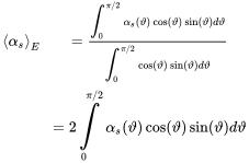
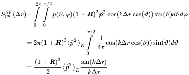
The global form of the cross correlation is also kept for half-space integration. Two locations at the walls of a diffuse field have the above correlation function. This expression is used in experiments to check the quality of the diffuse field, see e.g. Jacobsen (1979) for details.
6.1.5 Topology Conclusions
With the different dimensions comes different behavior regarding correlation and surface intensity. The relationship between energy density and the normal surface intensity can be described by a proportionality factor
This factor scales from for one-dimensional systems to and for two-dimensional and three-dimensional systems, respectively, as summarized in Table 6.1.
Table 6.1 Intensity and cross correlation depending on system dimension
| Dimension | Intensity | |
|---|---|---|
| 1D | ||
| 2D | ||
| 3D |
In Figure 6.5 the different cross correlation functions are compared to each other.

Figure 6.5 Normalized cross correlation functions of one- to three-dimensional diffuse reverberant fields. Source: Alexander Peiffer.
6.1.5.1 Dissipation in the Reverberant Field
In the reverberant field there are two processes for sources of damping: first, the damping during wave propagation, for example described by the complex wave number , and second, the absorption due to the reflection at an absorbing surface at end sections, edges, or surfaces. In principle, all systems have a volume, a one-dimensional beam or tube has a cross section, and plates have thickness.
According to (1.67) the loss due to wave propagation is given by
The dissipation due to surface absorption is given by the intensity irradiating all surfaces. The dissipated power due to boundary reflection in the diffuse field is
is the total and given by
is the perimeter area or boundary. In order to get an expression that fits to the global damping loss factor, the dissipation at the perimeter is expressed by the total energy of the random field.
The sum of both dissipations provides the effective damping loss factor
A random system with certain energy has a time decay so that without any power flow into the system the energy will decay as
6.1.6 Auto Correlation and Boundary Effects
The autocorrelation of the above given function follows from . Please note that this is
At the boundaries of such fields we have two effects. First, for the total sum of energy only half of the space is available. Thus, the mean square value of the amplitude is half of the amplitude if the full angle is available. Second the reflected wave amplitude is . So, the boundary amplitude of every ensemble wave is
In case of hard walls and fixed edges this means a doubling of the pressure or stress, leading to four times higher mean square value of the amplitude. This is partly compensated by the fact that only waves from half space can reach the boundary
The amplitude of each noncorrelated wave doubles for full reflection and (), but for the summation of all waves only half of the room, area, or line is available. In other words, the double amplitude is partly compensated by the fact that only half the space is available
Note, that one coherent wave would give twice the amplitude. The factor of instead of two in the reverberant field sometimes leads to confusion.
6.1.7 Sources in the Diffuse Acoustic Field – the Direct Field
Every system requires sources to get power input into the system. The waves that radiate from the sources or boundaries are obviously deterministic, because no reflection that may generate uncertainty has taken place. In the vicinity of the source around a radius of a few wavelengths there is a deterministic wave field with similar shape and behavior as in free field conditions as long as the wave amplitude reaches the diffuse field level. In room acoustics this distance is called the source radius. For correct measurement of the diffuse sound field level the distance between source and microphone must be larger than this radius. In the following examples, the direct field is included, except for the one-dimensional systems. The reason for this is that there is no geometrical attenuation for one-dimensional systems which is the case for two-dimensional () and three-dimensional systems ().
6.1.8 Some Comments on the Diffuse Field Approach
The considerations in Sec. 6.1.7 regarding the diffuse field are very stringent. The system must be constructed and uncertain in such a way that the reverberant field assumptions are met. Thus, the properties of the system must allow a large number of reflections with uncertain phase so that there are enough waves with equally distributed angles and random phase.
This is hard to achieve when the system is excited, for example, only at one point. Consequently, the diffuse field approach (and also the statistical energy method that is based on this concept) is of limited precision when local and single excitation occurs. So, when this is the case we should consider using deterministic and numerical methods for systems that are locally excited.
However, when many excitations exist the diffuse wave field can be applied. When the frequency is high enough for geometrical acoustics, this is one further option to be applied to random wave fields but allowing energy distributions along the systems described by random wave fields.
As mentioned at the start of this chapter, one approach is to average in addition over frequency bands. However, with the ensemble concept the properties of the reverberant field can be kept, so the more critical question is how large the variation from the mean value is and under which conditions the mean value fulfills the reverberant field assumptions. Please note, that also frequency averaging does not solve the issues regarding the strict diffuse field assumptions. In the remainder of Chapter 6, we will deal with some examples of random systems in order to explain these phenomena.
6.2 Ensemble Averaging of Deterministic Systems
In Sections 6.3, 6.4, and 6.5, we will numerically simulate ensembles of representative systems. Therefore, we take the response of acoustical or structural systems with slight variations of input parameters. When the deterministic response of one ensemble representation is given by , will represent a specific parameter set This could be the density , the Young’s modulus , or the thickness of a plate . In engineering systems this may also include local variations of those properties and the geometry.
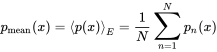
From this we get the ensemble averages
For we get the autocorrelation and
for the rms value. Even though the model conceptions of the reverberant field use uniform amplitude for all waves, the wavefield is not uniform for real systems. In order to capture this the space averages over the system extensions length, area, and volume are defined as follows
 (6.36)
6.3 One-Dimensional Systems
The investigation starts with a system dimensionality that is rarely used in the context of reverberant fields, because it is hard to imagine that a reverberant field builds up from back and forth reflected waves. However, when the one-dimensional system is large (compared to the wavelength) and there is uncertainty in the ensemble in terms of wave speed, length, and boundary conditions, even one-dimensional systems may by diffuse.
The advantage of one-dimensional systems is that fast and analytical solutions are available, and we can easily investigate all aspects of an ensemble of systems.
6.3.1 Fluid Tubes
Let us imagine that we have an ensemble of tubes with different temperatures and consequently variations in the speed of sound or small imperfections in length. This would lead to propagating waves with random phase for both directions if the imperfections and variations in sound speed lead to differences in the propagation paths exceeding one wavelength.
Those imperfections will cause a diffuse sound field in an ensemble of one-dimensional systems. The wave quantity is the acoustic pressure and the pressure field inside the tube is given by (4.24). Damping is introduced to ensure dissipation.
6.3.1.1 Energy
The reverberant pressure field is characterized be the mean square amplitude that is related to energy density of the wave and the total energy of the system. As the wave quantity is pressure, the constant in Equation (6.16) is .
Thus, the random state is defined by the energy density , the energy per length , or the total energy with a given length
In the diffuse field model the energy is equally distributed over the length. The irradiated intensity at both tube end cross-sections follows from (6.16)
6.3.1.2 Power Input to the Reverberant Field
The power input into the field is defined by Equation (4.20). For large values the radiation impedance of the system becomes a smooth function that approaches the impedance of a half infinite tube , and the resonance peaks disappear.
We would now like to present an instructive explanation for this effect using the modal response.
We consider the half bandwidth of one modal peak that is given by . One can expect a smooth frequency response when the distance between the modal frequencies is equal or smaller than the half power bandwidth because the modes are overlapping in this case. This relationship is quantified by the factor
So, we have two parameters to control the smoothness of the response (independent from random effects): The damping loss and the modal density . When the model overlap factor is larger than 1 we can estimate the power input into the system by Equation (4)
This effect is depicted in Figure 6.6. When the modal overlap factor is less than one the gap between the modes is large enough so that single peaks can be identified; when is approaching 1 there is still some waviness. For the slope of the power input is nearly constant. Note that there is no ensemble averaging involved – the only condition is that all modes are equally distributed over the frequency band.

Figure 6.6 Power input for various modal overlap factors. Source: Alexander Peiffer.
6.3.1.3 Dissipation
Surface dissipation occurs at the interaction with the tube end sections (neglecting the tube wall) with the total absorption area
With the tube volume and the combined dissipated power is
providing the effective damping loss factor.
6.3.1.4 Power Balance

Figure 6.7 Power balance for the one-dimensional tube system. Source: Alexander Peiffer.
In a stable configuration the input power equals the dissipated power. This is the birth of our very first and simple SEA model
Looking at the above equation we see that the input power depends on the free field impedance of the pipe on one side; on the other side, the loss of energy is proportional to energy and frequency given by the factor . With Equation (6.37), the rms pressure is then given by:
6.3.1.5 Energy Ray Tracing
For increasing frequencies, the wave attenuation (2.58) is getting larger, so the wave propagation is highly damped. Consequently, there are not enough reflections available to guarantee reverberance and an equal distribution of wave energy in the field. A description of random systems by diffuse wave fields is no longer valid, and methods that account for the damping along the propagation and system dimension are required.
The frequency limit of this effect can be estimated when we say that the energy damping along the system extension must not exceed , hence
Though SEA is often mentioned as a high frequency method, this important criteria for the application of SEA is neglected. If this criteria is not fulfilled, the error in the propagation of energy is not caused by an erroneous coupling of systems but the nonuniform energy distribution in the system. This issue can be overcome by geometrical acoustics. For very small wavelengths the wave propagation and scattering can be described by rays (Pierce, 1991; Kuttruff, 2014). Each wave is traced similar to the ray model in optics, and the wave field is considered as the sum of these rays. For a one-dimensional system, this can be done analytically.
We consider each propagation in the positive and the negative direction as one ray. We still assume a vibrating piston with velocity on port 1. A ray in the positive direction will radiate into the tube the mean squared pressure as follows
At the end of the tube, the wave is reflected with the reflection coefficient , so the reflected mean square pressure is
with ; this wave is reflected at port 1 with the coefficient and so on and on:
 (6.47)
The last term in parenthesis is an infinite geometrical series and we get for the slope of the root mean square pressure
6.3.1.6 Load at the Boundaries due to the Reverberant Field
The reverberant field will have an impact on the boundaries of the system. For deterministic systems the answer is given by Equation (4.24) or the pressure distribution itself. The field pressure at the boundaries creates a reaction force or pressure. The question now is what is the reaction force of a diffuse field that is only described by its energy or rms pressure average in the system?
The pressure in the diffuse field with energy is:
The ratio can be expressed by the modal density providing
According to Equation (6.31) the mean square pressure at rigid surface doubles
Finally, the auto spectrum of the blocked force that is generated by the diffuse field is given by
Here is the mechanical free field impedance of the one-dimensional tube.
We have compiled all the information required to describe a random system by a diffuse field. This includes the interaction of diffuse field at the boundaries with external systems:
- The input impedance of the reverberant field determining the power input.
- The load generated by the reverberant field at the boundary.
6.3.1.7 Monte Carlo Experiment
The applies uniform random variation to parameters of a system that is solved numerically. By this method a large ensemble of systems and its response can be simulated. The pressure field for a deterministic system is known from Equation (4.24) and therefore an excellent case for fast calculation of a large set of results that can be averaged. In order to work out the limits of the diffuse reverberant field we deal with two realizations of damping.
- Damping is dominated by dissipation in the wave propagation given by the complex wave number with and rigid ends.
- Damping is dominated by absorption at the boundary by applying an impedance leading to a reflection factor of . Damping loss for propagation is .
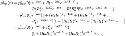
On the LHS of Figure 6.8 it can be seen that the system damping loss for case 2 starts with high values but is decreasing. The damping loss is defined per cycle, and for higher frequencies the wave passes many cycles before the reflection dissipates energy from the system. Thus, this case reaches a modal overlap of at and case 2 is not in the investigated frequency range.

Figure 6.8 Damping loss and modal overlap of both cases.
Source: Alexander Peiffer.
Those values are selected to investigate the statistical aspect and to reduce the effect of high modal overlap that would smooth even the deterministic response.
For ensemble realization, we randomize the speed of sound by and . We generate representations of this ensemble, with pressure and calculate the following ensemble averages:
 (6.53)
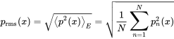 (6.54)
The first average shall show that the mean value vanishes in an ensemble average; the rms value should verify the reverberant field assumption for high frequencies. The spatial average over length will also be presented in the following numerical experiments to check if a single value can be representative for the total system.
6.3.1.8 Input Power and Impedance
From section 4.1.1 and the modal overlap discussions, it was shown that the radiation impedance approaches the free field impedance. This effect should occur even earlier in frequency due to incoherent reflection according to the diffuse field concept. In Figures 6.9 and 6.10 this effect is clearly visible for both cases. The light grey background represents the ensemble of different realizations.

Figure 6.9 Relative radiation resistance for an ensemble of tubes with 2% variation in and 1% in length, LHS rigid ends, RHS at port 2 with absorbing boundary conditions. Source: Alexander Peiffer.

Figure 6.10 Relative radiation reactance for an ensemble of tubes with 2% variation in and 1% in length, LHS rigid ends, RHS at port 2 with absorbing boundary conditions. Source: Alexander Peiffer.
For case 1 with dominating wave absorption the ensemble mean reaches very early () the free field limit with higher peaks in the ensemble variations. In case 2 the ensemble peaks are still quite sharp, because of the low modal overlap even for higher frequencies.
The same effect can be seen in Figure 6.10. The second case’s mean value oscillates more, but the ensemble variation is smaller.
Doing the same investigation with the input power, this is further confirmed. In Figure 6.11, the free field limit is reached much earlier than for the deterministic case shown.

Figure 6.11 Power input to an ensemble of one-dimensional acoustic tube systems LHS case 1 RHS case 2. Source: Alexander Peiffer.
6.3.1.9 Random Fields
We investigate the rms and mean pressure along the tube. The results are shown in Figures 6.12 and 6.13 for cases 1 and 2, respectively. Several modal frequencies and overlap factors are shown to investigate the validity and limits of the random field assumptions in both cases. For the first frequency, the main impact of the uncertainty is a large variation in amplitude, but each wave form remains stable in phase. So, mean and rms averages result in the similar pressure distribution along the pipe. This is still true to frequencies around the 10th mode as shown in the upper right axes. When we compare the rms pressure averaged over length to the result of the SEA model the agreement is quite good.

Figure 6.12 Monte Carlo simulation of an ensemble of tubes with speed of sound and length variation, case 1, , rigid ends. Source: Alexander Peiffer.

Figure 6.13 Monte Carlo simulation of an ensemble of tubes with speed of sound and length variation, case 2, , absorption at port 2. Source: Alexander Peiffer.
Reaching higher frequencies as shown in the lower left axis, both rms values don’t coincide, because damping along the tube prevents a constant pressure along the pipe. The mean pressure becomes zero for but not for near the vibrating piston side. Here, the coherence of the near field keeps the constructive interference near the source; the wave field has not yet gathered enough uncertainty to establish a diffuse sound field. This is the direct field component which can be added to the reverberant background to improve the precision of the sound field description.
For the high frequency results in the lower right axis it can be seen that rms pressure shows a strong decay along . The wave propagation is strongly affected by damping, and the diffuse field assumption is not met any more. It is the assumption of equivalent amplitude for both directions that is explicitly violated. The system is dynamically complex, but the damping is too high to establish a reverberant field. In this case ray-tracing or geometrical acoustics shall be applied, which agrees very well with the average result.
However, there are many options to achieve a reverberant field. Our case is very stringent, because there is only one source at one end of a one-dimensional field. If there are more sources, a reverberant field can be realized even for damped waves.
So, even with such a simple system the effects of deterministic and random regimes are visible. At low (deterministic) frequencies, there is the typical wave dynamics with maxima and minima regarding the related wave shape. The wave motion, the local minima and maxima, can be clearly determined. In the random regime the wave behavior is smeared out. In the statistical energy description, neglecting the phase is sufficient to describe the dynamics of a complex system. For higher frequencies when damping along the system dimensions becomes important, the damping must be considered, for example, by energy ray tracing methods. This high frequency limit is often neglected in the literature. Lyon and DeJong (1995) and Le Bot (2015) derived the same equation as (6.44) but expressing an upper limit of system size
For the power input the local dynamics of the area near the excitation must be known precisely, meaning that the free field impedance is required. Thus, even when we later deal with fully random models the dynamic properties of the system in the vicinity of junctions must be precisely known and is thus considered as deterministic.
6.4 Two-Dimensional Systems
The rectangular plates is taken as a test case for two-dimensional (2D) systems. The bending wave is dispersive and this impacts the diffuse field assumptions and the link between out-of-plane motion and the energy density.
6.4.1 Plates
We apply a point force excitation somewhere at the plate and focus on bending waves, because the wave speed for the other propagation modes is too high to create large modal overlap at audible frequencies even for large plates. Similar to the acoustic tube, the high modal overlap causes the mechanical impedance to reach the free field radiation value (3.226) of the infinite plate. The modal approximation is used to calculate the system response for the Monte Carlo analysis. Plates are two-dimensional systems; so, all equations for the two-dimensional wave field apply, and the field quantity is the displacement in the -direction.
6.4.1.1 Energy
In section 3.7.6.1, the energy per area is given by
providing energy density and energy by
Thus, the constant is
and for the two-dimensional expression of diffuse field intensity at the edges (6.18) we get
Please note that the intensity expression is per edge area – for intensity per length this expression must be multiplied with the plate thickness . In addition, the group velocity is different to the phase velocity and depends on the frequency
6.4.1.2 Power Input to the Reverberant Field
For systems and frequencies of high modal overlap the mechanical impedance converges to the free field impedance of an infinite plate. Thus, the input power can be calculated using the assumption (3.226)
However, the free field assumption is not fulfilled for low frequencies so we will use Equation (5.42) in addition to correct the power input.
6.4.1.3 Dissipation and Power Balance in the Reverberant Field
The same dissipation assumptions as for one-dimensional systems apply and the inert damping due to wave propagation is the same
For two-dimensional systems, the edge intensity is determined from our considerations in section 6.1.1, the volume is , and the dimensional constant is . The power balance provides the energy of the subsystem with given input power
with the average displacement result is
6.4.1.4 Direct Field Correction
For the direct field part in the vicinity of the point force, we add the results from Equation (3.231)
to the reverberant field.
6.4.2 Monte Carlo Simulation
The dimensions of the rectangular plate test case are m, m and mm. The ensemble is realized by varying the thickness by and the area mass by , and the system average response is presented by the rms displacement averaged over the plate area
6.4.2.1 Input Power and Impedance
In Figure 6.14 the mean value and the ensemble impedances are shown together with the modal overlap. Due to the properties of the plate, the modal density is constant over frequency (5.35); the consequence for the modal overlap is, that it increases linearly with frequency

Figure 6.14 Point impedance at m m with 2% thickness variation and 1% density variation and modal overlap over frequency. Source: Alexander Peiffer.
The modal overlap is above 1 around a frequency of s−1. Even though there is an ensemble average the input impedance of the free field is hardly approached. There is a remaining variability even at high frequencies. The reason for this is that the point excitation does not excite all modes equivalently. This is different to the tube case where we excited at the and thus made sure all the modes are excited. This is not the case for the plate. A mode that has zero amplitude at the point of excitation will not be excited and will not contribute to the statistics of the assumed random field. This is the reason why we also use the real input power calculated from (5.42) to correct the power input for the final random field comparison. It is worth mentioning that commercial software codes implement the point force in the same way leading to similar error. Thus, if the response of plate structures to point forces is targeted, the input power should be derived by alternative methods, e.g. experiments or modal methods as suggested above.
6.4.2.2 Random Displacement Field
When we do the random response analysis based on the power balance according to Equation (6.63) and the Monte Carlo analysis with the various random quantities, we get the result in Figures 6.15 and 6.17 for s−1 . The rms wave field shows still some variation even in the ensemble average. However, when we compare the displacement averaged over the surface, the order of magnitude is met, and the corrected power input leads to an improvement in the prediction quality.

Figure 6.15 Ensemble rms reponse of plate at s−1, dimensions m, m and mm. Source: Alexander Peiffer.

Figure 6.17 rms displacement along cuts in and -directions for s−1, dimensions m, m and mm. Source: Alexander Peiffer.
The assumptions of the diffuse field are better fulfilled at frequencies around s−1 as shown in Figures 6.16 and 6.18. The oscillation of the displacement rms still exists. But the SEA result and the surface average coincide very well. Here, the SEA random result plus the direct field component shows a much better agreement with the Monte Carlo result.

Figure 6.16 Ensemble rms reponse of plate at s−1, dimensions m, m and mm. Source: Alexander Peiffer.

Figure 6.18 rms displacement along cuts in and -directions for s−1, dimensions m, m and mm. Source: Alexander Peiffer.
6.5 Three-Dimensional Systems – Cavities
The first historical treatments on diffuse reverberant fields were in the context of acoustic fields in large spaces shown, for example, in Morse and Ingard (1968), Pierce (1991), or Jacobsen (1979). Diffuse acoustic fields are experienced in daily life – reverberant rooms can be found in many industrial or office spaces. The reverberant field in
churches can be so disturbing that speech recognition is not given, or music must be adapted to the special conditions.
Large rooms easily reach high modal overlap factors and modal densities at relatively low frequencies. This has led to many test set-ups and norms that apply reverberation chambers in order to experimentally create a standardized diffuse field excitation. Systems of solid materials rarely occur in transportation or even building constructions, and they can hardly be described by diffuse random fields due to the high wave speed of longitudinal and even transversal waves; those systems are simulated by deterministic methods. Thus, the only system we will deal with in the three-dimensional (3D) context are fluid cavities. Cavities meet the conditions of the diffuse field assumptions easily, but the upper SEA limit (6.56) is also often reached. So, ray tracing or optical methods can be used as in the tube example, because the ratio between wavelength and room dimensions are on the order of magnitude that allow for geometrical acoustics. For example, concert hall acoustics is an excellent case for the application of ray-tracing methods as described in Kuttruff (2014).
6.5.1 Energy and Intensity
The link between pressure field and system energy is given by
The intensity at the boundary is
The above expression is known as the irradiated intensity in a twin chamber arrangement where the average pressure is measured in the room. The power irradiating a specimen of surface at the room walls is
6.5.2 Power Input to the Reverberant Field
From section 4.2 and Equations (2.95) and (2.96) the radiated power is determined by:
The power input based on modal room theory is given by Equation (4.89)
6.5.3 Dissipation
The dissipation in room cavities depends on propagation and boundary absorption (6.41). For the surface absorption we must consider the angular dependency of the absorption according to Equation (2.103) related to the normal component of the intensity.
 (6.70)
with
Usually, the angular integration is performed numerically. Assuming that the room is surrounded by surfaces and with absorption the total follows from Equation (6.25), and the final dissipation formula (6.27) reads in case of cavities as
 (6.72)
6.5.4 Power Balance
The pressure in the room follows from the balance of energy flow
Similar to the considerations for the plate, the direct pressure field amplitude of the point source (2.91) is added to the random field component.
6.5.5 Monte Carlo Simulation
The test case applies the modal room acoustics from section 4.2 considering two different cases.
room 1 Damping is dominated by dissipation in the wave propagation with and rigid wall surfaces.
room 2 Damping is dominated by absorption at the boundary by applying an impedance at floor and ceiling leading to a diffuse field absorption coefficient and an absorption area m2. Wave damping is .
The ensemble variation of the room lengths is and for the speed of sound .
6.5.5.1 Room Absorption
In Equation (4.79), a complex wavenumber was introduced to determine the impact of absorbing boundaries on the modal coefficients. For nearly rigid walls, the off diagonal terms can be neglected and we get
Thus, we select and get specifically for the floor area the following expression
 (6.75)
When we evaluate expression (6.70) for the floor area we get for the average absorption coefficient for the floor leading to a total absorption area of m2.
6.5.5.2 Input Power and Impedance
Studying the ensemble average radiation impedance, the results from the sections before are further verified. The modal overlap becomes larger than one (Figure 6.19) above s−1.

Figure 6.19 Modal overlap for both rooms. Source: Alexander Peiffer.
Both real ensemble impedances (Figures 6.20 and 6.21) show resonance variation at low frequencies but approach the free field value. The modal peaks of room 2 are lower at low frequencies because of the larger modal overlap from the beginning, whereas the variations between each ensemble representation are higher for room 2 because of the lower damping contributions from the fluid.

Figure 6.20 Ensemble acoustic radiation impedance of room 1 and monopole ( m, m, m). Source: Alexander Peiffer.

Figure 6.21 Ensemble acoustic radiation impedance of room 2 and monopole ( m, m, m). Source: Alexander Peiffer.
6.5.5.3 Random Pressure Field – Room 1
The pressure field at lines passing through the source is shown in the Figures 6.22 and 6.23 for s−1. The need for near field consideration is further confirmed, but with this simple direct field consideration the random field pressure corresponds surprisingly well to the Monte Carlo result. At the boundaries the pressure is roughly higher than the field pressure as predicted by Equation (6.31). Due to the high expense of the calculation time, only 100 averages were performed leading to limited statistics.

Figure 6.22 Ensemble pressure field in rectangular room 1 ( m2) along -line through source location (). Source: Alexander Peiffer.

Figure 6.23 Ensemble pressure field in rectangular room 1 ( m2) along and -lines through source location (). Source: Alexander Peiffer.
6.5.5.4 Random Pressure Field – Room2
At 5000 s−1, the second room with damping via absorption shows a similar agreement between random and the Monte Carlo results (Figures 6.24 and 6.25). The suitability of three-dimensional systems for reverberant field modelling is further verified.

Figure 6.24 Ensemble pressure field in rectangular room 2 ( m2) along -line through source location (). Source: Alexander Peiffer.

Figure 6.25 Ensemble pressure field in rectangular room2 ( m2) along and -lines through source location (). Source: Alexander Peiffer.
6.6 Surface Load of Diffuse Acoustic Fields
The reflection of the diffuse wave field at the room boundaries creates random load at the boundary surfaces. The amplitude doubles due to Equation (6.30) for each room angle . The cross correlation spectrum at the surface is derived by the integration over half the room angle. Modifying (6.21) accordingly reads
 (6.76)
This is in line with the discussion in section 6.1.6. The pressure at the boundary is called the blocked pressure (force) when the walls are rigid and we have total reflection (. In the random description of subsystems global quantities such as volume, energy, and the modal density are given. Expressing the field pressure in these terms gives
With the modal density of rooms and when perimeter and surface effects can be neglected we get
Entering this into (6.76) we get for the cross correlation of the diffuse acoustic field with energy and modal density
When we discretize the surface by a regular mesh with element area , the cross correlation of the blocked force load is
Note that the grid length in this mesh must be much smaller than the wavelength. The sinc function in the above description can be replaced by a more generic expression. The transfer impedance of one vibrating element at to another element located at is given by the Rayleigh integral of the semi infinite half space with rigid wall (2.141) and constant velocity over the small element area.
and the transfer impedance for the mesh is
providing a mechanical impedance when we multiply the acoustic impedance by . The real part of this provides the wanted sinc function
Entering this into (6.80) we get the diffuse field reciprocity relationship for acoustic wave fields:
This is an important and useful expression. We can determine the cross spectral load function of diffuse fields only from the total energy, the modal density, and the real part of the radiation impedance. Thus, the response of every deterministic system described by a transfer matrix and that is excited by a diffuse acoustic field can be calculated using the matrix multiplication from section 1.7.2.
This expression was proven by Shorter et al. (2005) for general diffuse wave fields. So, the response of any deterministic system excited by a reverberant field can be calculated using the above expression.
6.7 Mode Wave Duality
For the investigation of the diffuse field concept applied to ensembles of random systems, modal solutions of two- or three-dimensional systems are used. It seems that the modal description in combination with high modal density is a further appropriate model for reverberant wave fields, but we have not established a clear theoretical relationship between the modal and wave concepts. Lyon and DeJong (1995) investigated a system described by modal response with uncertainty in order to prove that the result from the diffuse wave field model can also be shown using the modal approach.
6.7.1 Diffuse Field Energy
In the diffuse field model with equal power from all directions, the homogeneous energy distribution is evident. For systems described by modes, it is not that obvious that modes (with a specific uncertainty) lead to an equally distributed mean square amplitude in the wave field.
6.7.2 Free Field Power Input
In the discussions of the modal overlap factor of section 6.3.1.2 we have established the criteria that allows treating the point impedances of resonant and deterministic systems as free field impedances. In that case the damping is so high that no reflection is received at the point of excitation (independent from the fact of whether the reflection is coherent or not).
We will now show that the free field assumption, which is easy to explain in the diffuse wave field model, can also be proven when we assume a Gaussian orthogonal ensemble of modes (see details in Langley (2016)). In this approach, the uncertainty in an ensemble of systems leads to small variations in the modal frequencies as shown in Figure 6.26 for one ensemble representation. When dealing with structural systems, the input power into the system excited by a harmonic source at a specific location and frequency is according to (1.49)
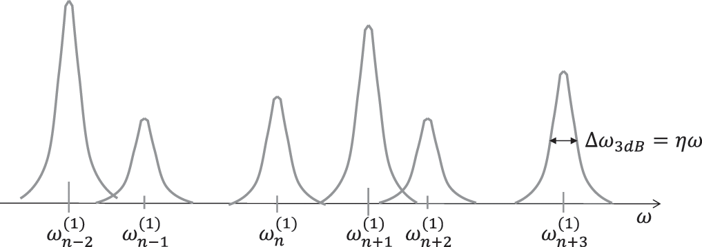
Figure 6.26 Distribution of modal frequencies near and the receptance function along the frequency axis for one ensemble representation. Source: Alexander Peiffer.
The real part is called, the imaginary part. For the derivation of the conductance of modal systems we take Equation (5.42) as a typical example.
In principle, every closed dynamic system can be described by the above equation. Independent from the fact of whether a discrete or homogeneous aproach is selected. In order to assess the real and imaginary parts of the mobility we rationalize the denominator.
and the conductance reads as
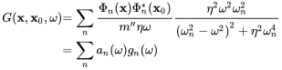 (6.88)
with , and that can be further simplified assuming that the major contribution is for frequencies near the resonances .
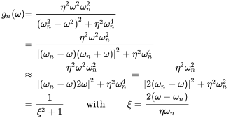 (6.89)
We stay first with one mode and investigate the ensemble average of of modal frequency . When the modal frequencies are equally distributed over the frequency interval the probability density of in this interval is as shown in Figure 6.27. Thus, the expected value of is

Figure 6.27 Ensemble of modal frequency distributions for one specific mode of frequency . Source: Alexander Peiffer.
This interval must be larger than the modal bandwidth for getting a smooth average, or in other words, the variation in modal frequency must be so large that the peak in frequency is shifted such that every value of is possible.
The sum over all is approximated by the number of modes times . is simply the product of the frequency interval and the modal density. Thus, the expected value of (6.88) is
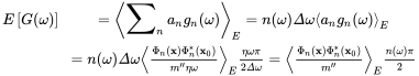 (6.91)
6.7.2.1 Point Conductance
For the point conductance, excitation and response points are the same , and the ensemble average over the sum of all modes is given as
The mode shape function from (5.33) is
Similar to the diffuse wave field, we assume that the mode shapes are not correlated. So, arguments in the sine functions in an ensemble of mode shapes have uncorrelated phase, and we take the expected value of each squared sine function . Thus,
and finally
When we use the modal density for a flat plate (5.35), the result is
which corresponds exactly to the point impedance of infinite plates (3.226). We can conclude that for an ensemble of modal systems with modal frequency uncertainty with stable modal density and frequency variation , the point conductance and also the impedance are equal to the free field expression.
6.8 SEA System Description
Random subsystems are described and modelled by a few properties that characterize the random field. These are geometrical entities such as volume, area, and length. In addition, the ratio of these quantities to the boundaries is also important. This determines the modal density, therefore the modal overlap that allows estimating when the wave field can be assumed as a diffuse random wave field. The power input into the systems is determined by the free field impedance.
The power loss due to damping of the systems may be caused by dissipation in the wave propagation or absorption at the system boundaries. From the power balance, the energy state of the system can be calculated. Once the energy is computed, the wave field property can be recovered from the link between energy density and each appropriate engineering unit, e.g. pressure, displacement, and velocity.
Thus, a complicated and detailed system is reduced to a small set of global parameters that allow simple determination of the random system response. This is the reason why SEA is very practical when dealing with large systems of high dynamic complexity and uncertainty.
However, the diffuse field assumption has its limitations, especially when it comes to large propagation damping. In this case, methods similar to optics may be applied that consider effects of damping and diffraction or shadowing of wave fields.
6.8.1 Power Balance in Diffuse Fields
In the introduction to Section 6.8, the model of the diffuse acoustic field was applied to describe the state of a dynamically complex system, as shown in Figure 6.28. For the single system, the equation is simple, and the energy of the system that determines the amplitude of pressure, displacement, or other wave amplitudes is given by

Figure 6.28 Single SEA system power flow. Source: Alexander Peiffer.
Engineering systems consist of several components and systems. Therefore there are usually many diffuse acoustic fields (encapsulated in specific systems) that are exchanging energy. This transmitted energy is related to the system surface intensity as given by Equations (6.16), (6.18), and (6.20) as far as the connecting area and the transmission of radiated waves into the other connected subsystems. The details of this coupling will be discussed in Chapter 7. In the following we use the upper index for the th subsystem for quantities that are already using a descriptive index as for example , .
In Figure 6.29, two connected random systems are depicted. In order to cope with the damping loss , we use a similar expression for the loss due to transmission into the connected subsystem. Thus, the power transmitted by subsystem into system reads as

Figure 6.29 Two connected SEA systems power flow. Source: Alexander Peiffer.
The expression for the other direction is
The coefficient is called in accordance with the definition of the loss factor. The total power balance for subsystem (1) is
and for subsystem (2)
When we consider a number of subsystems the power balance of the th subsystem would be given by
and this can be written in full matrix form as
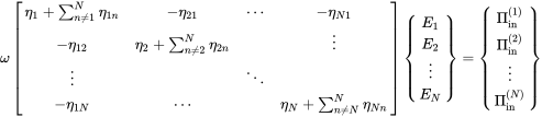 (6.102)
or in short form
is called the power-flow matrix or the SEA matrix.
6.8.2 Reciprocity Relationships
Reciprocity is a general principle that relates the conjugate input variables of a two port system. Applied to the mechanical systems of Chapter 5, that means that the velocity at position 1 generated by a force at position 2 is similar to a velocity at position 2 generated by the same force at position 1. This general principle applies to all systems that are composed of linear, passive, and bilateral elements.
The same principle must be fulfilled for random systems. Thus, if we apply a force at system 1, the velocity response at system 2 at one point and therefore also at the average must be similar to the reciprocal configuration – that is, the force excitation at system 2 and the velocity response at 1.
Now imagine a two system SEA configuration as given by Equation (6.99). When the force is exciting exclusively system 1 (), the solution of this system with regards to the energy of system 2 is
and a similar solution is found for the excitation at subsystem 2
The reciprocity relationship must now be converted into energy and power expressions. The energy of the subsystem is given by the total mass and the average velocity of the subsystem
and the power input is determined by the conductance
When expressing power and energy by the above expressions and squaring the reciprocity relationship (6.104) we get
This leads to an expression that relates the SEA matrix coefficients using conductance and mass quantities.
In section 6.7.2 a relationship for the input conductance that links the input power created by force excitation and the modal density was found
leading to
This is the reciprocity relationship of SEA and it leads to a symmetric form of the equation when dividing each energy by the modal density of the system. When we define the double index for the damping loss, we may write
 (6.113)
This matrix is symmetric and better suited for computationally efficient solvers. In addition, only half of the coupling coefficients must be determined. We denote this symmetric matrix with
6.8.3 Fluid Analogy
The principle of energy per modal density motivates the fluid analogy of SEA shown in Figure 6.30. The amount of water corresponds to the total energy in each subsystem, the width to the modal density (linearly dependent on the number of modes in band), and the height of the fluid in the tank is the energy per modal density. The power input and losses are the amount of fluid per time that are entering or leaving the systems. The exchange of fluid depends on the energy difference in the systems.

Figure 6.30 Fluid analogy of SEA. Source: Alexander Peiffer.
6.8.4 Power Input
The input power is determined from the source properties and the convenient property describing the reaction to this excitation. When we studied the different random systems we showed that in the ensemble average the dynamics of the system is equal to the free field radiation dynamics of the involved wave physics. In other words: sources connected to a random system get the dynamic reaction of the free field. This fact is quite obvious in the model construct of the diffuse wave field model, because it is one main assumption of this model that there is no coherent reflection from the boundaries of the diffuse wave field system. But, even in modal space this assumption can be proven given the right statistics and uncertainty for the involved modes. When damping is high enough, this fact can even by shown without any ensemble averaging. In this case, the reflecting waves are simply damped out.
Thus, the important message is that random systems have the same dynamic characteristics as the according free field. Assuming a surface impedance of a random system, the ensemble average of the free field radiation impedance is supposed to be
6.8.5 Engineering Units
The random description of systems involves the energy of systems but not directly the required quantity. In general we must separate between the potential and the kinetic energy of the waves, but as the model of the diffuse field is linked to the propagation of plane waves, we can use the statements from the plane wave energy descriptions: the potential and kinetic energy is equally distributed, and we chose the typical wave quantity usually taken to describe the system.
For fluid systems such as pipes and cavities, this quantity is the acoustic pressure (6.37):
and for plates it is the displacement (6.57):
For practical reasons and better scaling over the frequency range, the results are often expressed as velocity or acceleration
The same can be done for one-dimensional system such as beams and pipes. For pipes the first equation applies; but, concerning beams and rods, we will not enter deeper into the details of random modelling, because the high bending stiffness in engineering systems (this is what their task is in typical constructions – to be stiff and to carry loads) doesn’t make random modelling of such systems realistic. In most practical cases, those systems must be considered as deterministic.
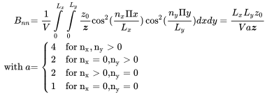
Table 6.2 Modal densities for one-, two-, and three-dimensional subsystems
| Dimension type | Modal density |
|---|---|
| Bars, rods, beams, pipes | |
| Plates, shells, thin cavities | |
| Cavities |
In the introduction to Chapter 6, we mentioned the ratio between wavelength and the dimensions of the subsystems as possible criteria to seperate between random and deterministic systems. Either the modal overlap must be greater than one, or the ensemble variation in modal frequency must be large enough to make the modal responses overlap to allow for a random description of the system. In all cases the major criteria is the modal density in combination with the damping as a factor in the first case or the frequency variation in the second case. To establish the link between the Helmholtz number , it is helpful to present the modal density in terms of the. Usually is linked to the phase velocity, but we set to allow for simple expressions that are used here as fuzzy criteria to separate between random or deterministic systems.
For the different exponents of the Helmholtz number, we assumed that and . With this view it becomes clear why two- and especially three-dimensional systems become random much earlier in frequencies than one-dimensional systems.
6.8.6 Multiple Wave Fields
In plates, there occur different wave types: the longitudinal, the shear, and the bending wave. In beams, there are even more types of wave propagation that are not treated in detail here. Those waves have different wavelengths, so there can be simultaneous waves that fulfill the requirements for a reverberant field and that do not. From the energy perspective, we may use a combination of wave types to describe a random system. It is good practice to consider the one wave type field as one SEA subsystem and not all wave fields in one system. We will see later that the calculation of the coupling loss factors will motivate a particular wave field selection. For fluids, the situation is simple, because there is only one mode of wave propagation.
Bibliography
- Finn Jacobsen. The diffuse sound field. Technical Report 27, Danmarks Tekniske Universitet (DTU), Lyngby, Denmark, 1979.
- Heinrich Kuttruff. Room Acoustics, Fifth Edition. 2014. ISBN 978-1-4822-6645-0 978-0-203-87637-4.
- R.S. Langley. On the statistical properties of random causal frequency response functions. Journal of Sound and Vibration, 361: 159–175, January 2016.
- Alain Le Bot. Statistical Energy Analysis, July 2015.
- R.H. Lyon and R.G. DeJong. Theory and Application of Statistical Energy Analysis, Second Edition. Butterworth Heinemann, 1995. ISBN 0-7506-9111-5.
- P.M.C. Morse and K.U. Ingard. Theoretical Acoustics. International Series in Pure and Applied Physics. Princeton University Press, 1968. ISBN 978-0-691-02401-1.
- Allan D. Pierce. Acoustics - An Introduction to Its Physical Principles and Applications. Acoustical Society of America (ASA), Woodbury, New York 11797, U.S.A, one thousand, nine hundred eighty-ninth edition, 1991. ISBN 0-88318-612-8.
- P. J. Shorter and R. S. Langley. Vibro-acoustic analysis of complex systems. Journal of Sound and Vibration, 288(3): 669–699, 2005.
- P. J. Shorter, Y. Gooroochurn, and B. Rodewald. Advanced vibro-acoustic models of welded junctions. In Proceedings Internoise 2005, Rio, Brasil, August 2005.