
8
Distillation Column Control
Steady-state simulation and design methods for separation processes, with emphasis on distillation, have been presented in detail in many references, a few of which are listed in the references for this chapter. This chapter will present a discussion of the basic control schemes for distillation columns. Let us start by stating the obvious: the amount of literature on separation processes, particularly distillation is colossal. Particularly readable books and references are those by Buckley [1,2], King [3], Tyreus [4], Seborg et al. [5], Shinskey [6], Smith and Corripio [7], Svrcek and Morris [8] and Wilson and Svrcek [9].
8.1 Basic Terms
When determining the control system design for a multivariable process, the terms control strategy, control structure and controller structure are used interchangeably. In this context, the meaning is the selection and pairing of manipulated and controlled variables to form a complete, functional control system. However, the three terms can also have individual meanings. Control strategy can describe how the control loops in a process are configured to meet a given overall objective such as the purity of a given stream. Control structure, on the other hand, is the selection of controlled and manipulated variables from a set of many choices. Finally, controller structure means the specific pairing of controlled and manipulated variables by way of feedback controllers.
This chapter will describe a methodology for designing a multivariable control system that includes elements of control strategy considerations, control structure selection and variable pairing. The methodology is largely empirical and based on general principles for distillation control. The methodology for control system design assumes that the process configuration is fixed and that changes are not possible. This is the case in many instances where control engineers are asked to design the control system for process configurations in an existing plant or a plant well into the design phase. The task for the control engineer is to select appropriate variables to be controlled and design controllers that will tie these variables to the control valves (manipulated variables) in such a way that the resulting controller structure meets the desired objectives. The final assumption is that the controller structure will be built up around conventional PID controllers, ratio, feedforward and override control blocks found in all commercial distributed control systems (DCS).
8.2 Steady-State and Dynamic Degrees of Freedom
When a process engineer works with a detailed steady-state simulation of a distillation column, a certain number of variables have to be specified in order to converge to a solution. The number of variables that need to be specified, or degrees of freedom, can be determined through the concept of the description rule as stated by King [3]:
In order to describe a separation process uniquely, the number of independent variables which must be specified is equal to the number which can be set by construction or controlled during operation by independent, external means.
Applying the description rule to a distillation column with a total condenser and two product streams gives two steady-state degrees of freedom. In this case the column would require two specifications, that is, a composition and a component recovery. The steady-state simulator will then manipulate two variables, such as reboiler and condenser duties, in order to satisfy the specifications and close the steady-state material and energy balances. If a partial condenser is added to the column, another degree of freedom is added to the steady-state column. Likewise, for each additional side draw added to the column, a new degree of freedom is added, requiring another specification.
When the same two-product distillation column is viewed in dynamics, the number of degrees of freedom increases from two to five. These three new dynamic degrees of freedom correspond to three new manipulated variables needed to control the integrating, inventory variables within the column that are not fixed by the steady-state material and energy balances alone. The inventory variables for this column are condenser level, reboiler level and the column pressure.
There are restrictions on the control of a distillation column. The overall enthalpy balance limits the heat removed by the condenser and added by the reboiler. The rate of distillate produced may not exceed the feed rate. The number of stages in the column and the reflux ratio must be greater than or equal to the number required for the desired separation [3].
One control valve (or degree of freedom) must be used for each controlled variable. This relationship between controlled variables and degrees of freedom (or control valves or manipulated variables) is known as variable pairing and is an important concept in control system design.
When the five manipulated variables, which correspond to five valve positions as shown in Figure 8.1, are viewed, it can be seen that the two steady-state-manipulated variables are a subset of the overall five. However, there is nothing about the heat duties that make them exclusive steady-state manipulators and prevent them from being used for inventory control. In many control schemes, the condenser duty is used for pressure control rather than composition control. For the same reason, any three of the five manipulated variables can be used to control the column inventories.
Figure 8.1 Basic distillation column schematic.
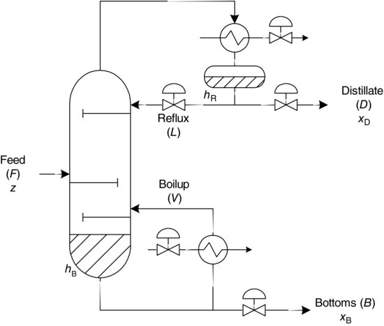
Although the previous paragraph describes the manipulated variables as control valves, there are many choices available other than just the individual valves. For example, many columns have reflux ratio as a manipulated variable for either inventory or composition control. When ratios and linear combinations of variables are included, the choice of a manipulator for a given loop broadens considerably for a simple two-product column. However, the steady-state and dynamic degrees of freedom remain unchanged as two and three, respectively, totalling five.
One must take care in determining the number of steady-state and dynamic degrees of freedom for more complex columns. Tyreus [4] describes the determination of the degrees of freedom for an extractive distillation system and for an azeotropic column with an entrainer. In the case of an extractive distillation system, recycle streams reduce the dynamic degrees of freedom through an increase in the steady-state degrees of freedom if the recycle contains a component that neither enters nor leaves the process. As well, if it is important to control the inventory of a trapped component, such as an entrainer for azeotropic distillation, it is necessary to provide extra control valves to account for the loss of degrees of freedom. The loss comes from the addition of a side stream.
In summary, the total degrees of freedom for actual plant operation equal the number of valves available for control in that section of the plant. To find out how many integrating variables, that is, pressures and levels, are to be controlled with the available valves, subtract the degrees of freedom required for steady-state control from the total degrees of freedom.
8.3 Control System Objectives and Design Considerations
Defining and understanding the control system objectives should be a collaborative effort between process engineers and control engineers. Left to either of these contributors alone, the objectives can be severely biased. The control engineer might be tempted to make the control system too complex in order for it to do more than is justified based on existing disturbances and possible yield and energy savings. On the other hand, a process engineer might underestimate what process control can achieve and thus make the objectives less demanding. It is crucial to define what the control system should do as well as to understand what disturbances it has to contend with.
Process understanding is another key, but often overlooked, activity for successful control system design. In practice, more time is spent on designing and implementing algorithms and complex controllers than on analysing process data and understanding how a process really works. Modelling and simulation are integral parts in the process understanding step.
Rigorous dynamic simulation is the third important activity in control system design. A flexible dynamic simulator allows for rapid evaluation of different control structures and their response to various disturbances. In choosing a control scheme there are several design considerations to take into account. First it is important to remember that a distillation column performs two basic functions:
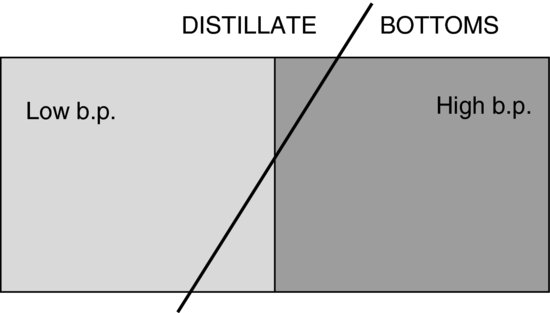
The feed split is the primary point of separation between the overhead and bottoms product. Fractionation is determined by the number of separation stages in the column and the energy input. Figure 8.2 illustrates these concepts with a mixture of a low boiling point component (light shading) and a high boiling point component (dark shading). The boiling point of the distillation products is determined by how much of each component is present in each product. As the distillation feed split changes, the line will shift left or right. As the fractionation changes, the slope of the line will change with a steeper slope representing better separation. It is important to realize that fractionation increases the purity of both products simultaneously while changing the feed split will make one product more pure and the other less pure.
Figure 8.2 Feed split and fractionation.
Once the inventory variables are controlled there are two degrees of freedom left in the case of the column shown in Figure 8.1. One degree of freedom should be used to control the feed split while the last available degree of freedom controls fractionation. Feed split has a much more significant effect on the product compositions than fractionation. Therefore, after the inventory and capacity variables have been paired, the primary controlled variable is normally used to set the feed split while the secondary controlled variable is used to set fractionation.
The following equations describe how the various manipulated variables are related and show that virtually any variable pairing can be used to achieve the desired control objectives. However, some pairings will provide significantly better sensitivity and responsiveness. Better sensitivity means that the control scheme will react with smaller changes, whereas a more responsive control scheme reacts more quickly.
Overall material balance:
Component balance:
where F is the feed; B is the bottoms; D is the distillate; xi is the concentration of a particular component in the feed, distillate or bottoms; Qreb is the reboiler duty; and Qcond is the condenser duty.
Energy balance:
where Hf is the enthalpy of the feed; Hb is the enthalpy of the bottoms; and Hd is the enthalpy of the distillate.
Combining Equations 8.1 and 8.2 to eliminate B or D gives
The control system must satisfy Equations 8.1 and 8.3 at all times. For particular values of xD and xB (i.e. composition specifications), Equation 8.4 or 8.5 also has to be satisfied. D, B, Qreb and Qcond can all be fixed or adjusted dynamically by control valves on the flow rate or utility streams. The reflux flow can also be adjusted dynamically and will directly affect the energy balance.
One of the most difficult aspects of distillation column control is the interaction effects between the material and energy balance and composition controls. Depending on the inventory controls, heat input or removal can alter both the material draws and the compositions. This interaction can work for us or against us depending on the control strategy.
Another point to consider when choosing a column control scheme is that typically the process gains from a high purity separation are very non-linear. This can be verified by simply using the component balance equations. For example, Equation 8.4 can be rearranged and differentiated at constant xB to give
Equation 8.6 shows that changes in the distillate rate, D, will have a much larger effect on the distillate composition, xD, when the distillate rate is relatively low as compared with cases when the distillate rate is relatively high.
A final and important consideration to keep in mind is the dead time that may be present in the column. In Chapter 3 dead time was described as being generated by a series of lags (material or energy capacitances). It is easy to see how a distillation column with its multiple stages can generate dead times. The control scheme on a distillation column should be set up to minimize the dead times with respect to the process lags and disturbances.
The steps for determining a suitable controller structure are as follows:
Ultimately, the importance of process control is seen through increased overall process efficiency allowing the plant engineer to get the most from the process design. This is especially true of distillation control. Most distillation columns are inherently flexible and a wide range of product yields and compositions can be obtained at varying levels of energy input. A key requirement of any control system is that it relates directly to the process objectives. A control system that does not meet the process objectives or produces results that conflict with the process objectives does not add value to the process.
8.4 Methodology for Selection of a Controller Structure
The economic performance of a distillation system is linked to its steady-state degrees of freedom. In other words, the economic benefits of a column control scheme depend on how well it controls composition, recovery or yield and not on how well it holds integrating variables such as levels and pressures. The integrating variables must obviously be controlled, but their control performances do not directly translate into profits. However, inventory controls can be the most troublesome of all loops and can preoccupy the operators to the point where the economically important composition and recovery are neglected. This problem has been resolved by designing the level and pressure controls before dealing with the composition controls [2]. However, one must be careful in the selection of the manipulated variables for inventory control as they can significantly impact the control performance of the composition loops.
The following methodology [4] can be employed to define a control structure for a simple distillation column shown in Figure 8.1:
For the simple distillation column in Figure 8.1, there are five degrees of freedom, which translates into five independent valves from a control point of view. In this 5×5 system, there are 120 possible single input/single output (SISO) control combinations of controlled and manipulated variables. Fortunately, most of these combinations are not useable due to various constraints, such as economics. From a steady-state degree of freedom analysis there are only two degrees of freedom, since a total condenser is assumed. If the column had a partial condenser there would, of course, be three degrees of freedom instead of two. Inventories that must be controlled are the reflux drum level (hR), level in column base or reboiler (hB) and the column pressure (vapour hold-up). The remaining two variables are used to control the feed split and the fractionation.
The feed split is simply the amount of feed that leaves as distillate versus the amount that leaves as bottoms. The other variable, fractionation, is the amount of separation that occurs per stage. The overall column fractionation depends on the number of stages, the energy input and the difficulty of separation. A typical control scheme for this column is shown in Figure 8.3.
Figure 8.3 Column basic control scheme.

The most convenient method of verifying the operability of a proposed multivariable control scheme is through dynamic simulation. However, to effectively use dynamic simulation it is first necessary to define the objectives of the control system, define the nature of the expected disturbances and develop a basic understanding of the process in terms of both its steady-state and dynamic behaviour.
8.5 Level, Pressure, Temperature and Composition Control
Measurement of fractionating column variables must be within certain tolerances of accuracy, speed of response, sensitivity and dependability; they must also be representative of the true operating conditions before successful automatic control can be realized. The instrument equipment selected, the installation design and the location of the measuring points determine these requirements.
This section is concerned with selecting the specific location in a fractionating column of the measuring points that will provide the best automatic control under variable process operating conditions. Specifically, level, temperature, pressure and composition measuring points in conventional fractionating columns are discussed. It should be clearly understood that this discussion, which is general in nature, is intended only to serve as a guide, from which detailed recommendations may be formulated and tested through dynamic simulation.
Locating temperature, pressure, flow and composition measuring points for automatic control systems depends on the control scheme used and the static and dynamic interdependence of these variables. The control scheme utilized is usually determined by the source of energy or process stream to be manipulated to control a particular variable. It is therefore important to consider the static measuring sensitivity of the instrument selected to measure the controlled variable. Measuring sensitivity should generally increase with requirements of control precision by the use of narrow-span suppressed range instruments. In addition, the location of the measuring element with respect to the energy source and the time lag involved for it to sense effects of changes in manipulated variables will determine dynamic measuring lags introduced by changing process conditions. The dynamic measuring lags will determine the quality and stability of the control scheme.
The interaction of temperature, pressure and composition will differ with location in the column. The selection of a temperature control point in a fractionating column, which is determined assuming that the pressure and composition are constant, may be unsatisfactory when these variables are permitted to vary with changing process conditions, that is, feed composition changes. The complex effect of all of the sources of disturbances in the form of changing process conditions on the measuring point must be considered for dynamic stability via dynamic simulation.
8.5.1 Level Control
Level control was discussed in detail in Chapter 7 in the liquid level control section. Typical hold-up times for condenser accumulators and reboilers are of the order of 5–10 minutes and 20 minutes (large enough to hold all the liquid from the trays if dumped), respectively. From a common sense point of view, to assign manipulative variables for level control, simply choose the stream with the most direct impact. For example, in a column with a reflux ratio of 100, there are 101 units of vapour entering the condenser and 100 units of reflux leaving the reflux drum for every unit of distillate leaving. Therefore, the reflux flow or vapour boil up should be used to control the drum level. If this assignment principle is not followed and distillate flow is selected for level control, it would only take a change of slightly more than 1% in either vapour boil up or reflux flow to saturate the drum level controller and saturate the distillate valve. The Rule of 10 can be applied. This rule states that if there is a 10 to 1 or greater difference, say reflux versus product, then the larger stream must be used to control the level.
8.5.2 Pressure Control
Pressure control is a primary requirement for all towers because of its direct influence on the separation process. Columns are typically designed to operate at sub-atmospheric, atmospheric or above atmospheric pressure. Tower pressure control configurations can also be required to vent varying amounts of inerts from the overhead accumulator. The venting of inerts or maintaining the desired operating pressure is often the crux of the control problem.
The same general principle is followed when finding manipulated variables for pressure control as for level control. Column pressure is generated by boil up and is relieved by condensation and venting. To find an effective variable for pressure control, it is necessary to determine what affects pressure the most. For example, in a column with a total condenser either the reboiler heat or the condenser cooling is a good candidate for pressure control. On a column with a partial condenser, it is necessary to determine whether removing the vapour stream affects pressure more than condensing the reflux. Sometimes the dominating effect is not obvious. If the vent stream is small, it might be assumed that the condenser cooling should be manipulated for pressure control. However, if the vent stream contains non-condensables, these will blanket the condenser and affect the condensation significantly. In this situation, the vent flow, although small, is the best choice for pressure control.
Figure 8.4 shows a typical pressure control scheme for sub-atmospheric column operation used for total condensing service. The eductor is not controlled by regulating the motivating steam, because the turndown on the jets is very limited. Rather, the capacity is controlled by regulating the addition of non-condensable gas. This method provides a smooth and rapidly responding control system.
Figure 8.4 Pressure control for sub-atmospheric operations.

Figure 8.5 shows a typical control scheme used for an atmospheric or above atmospheric tower in a total condensing service with little or no inerts. In this situation the pressure is controlled by regulating the flow of the coolant, which in turn changes the condensing surface temperature and the vapour condensing rate. The pressure response of this scheme to changes in the coolant flow rate is inherently slow in comparison to methods regulating vapour withdrawal directly and/or condenser surface area control.
Figure 8.5 Pressure control for above atmospheric operation.

Figure 8.6 shows a scheme where column pressure is controlled by regulating the flow of the vapour product from the accumulator. The reflux is on flow control. A level controller is required to control the coolant flow in order to maintain accumulator liquid inventory. This method provides a smooth, rapidly responding column pressure control.
Figure 8.6 Pressure control by control of overhead product vapour flow.

In Figure 8.7 column pressure is controlled by regulating the inert and vapour flow from the accumulator. The condenser coolant is fixed at a constant flow rate and should not be subject to change. A flow controller fixes the reflux rate while a cascade (level to flow) is used to adjust the product overhead rate. This cascade arrangement isolates the overhead product flow from internal column pressure disturbances that could affect the overhead product flow rate. Cascade control is only used if minimization of overhead product flow rate is critical to downstream unit operations.
Figure 8.7 Pressure control by venting of inerts.

For a total condensing service the column pressure can be controlled by varying the condenser level or the condenser surface area exposed to the column overhead vapours, as shown in Figure 8.8. The accumulator pressure and reflux temperature can also be controlled by providing a condenser vapour bypass or by controlling the coolant flow rate.
Figure 8.8 Pressure control by condenser level control.

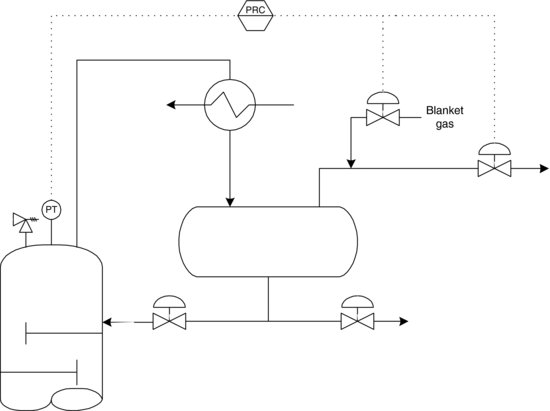
In a total condensing service, when varying quantities of inerts are present in a pressurized tower, it is often necessary to vent or alternatively inject a blanketing inert gas. This is normally accomplished using a split range control scheme, as shown in Figure 8.9. The column pressure is controlled by either injecting or venting blanketing gas from the accumulator/condenser.
Figure 8.9 Pressure control by regulating condenser surface area with blanket gas.
The location of a column pressure control point is not restricted by dynamic considerations. The response time of pressure changes in a column and the dynamic measuring lag has been found to be equally fast for any location in the column when the manipulated energy source used to control pressure is either condenser cooling or reboil heat. Pressure is regulated at a constant value and is rarely used as a variable to control a product specification. Generally, temperature is used to control composition, making pressure compensation necessary to sustain accurate control. Fractionation is affected by changes in the relative volatilities of the components due to variations in pressure. A decrease in pressure may cause the feed to flash, resulting in two-phase feed and column flooding [10].
Some of the factors that should be considered in locating the pressure measuring point are as follows:
8.5.3 Temperature Control
Composition control of products from a column is usually realized via temperature control. Temperature sensors are inexpensive, highly reliable, repeatable, continuous and fast compared to composition sensors [11]. The measurement lag is particularly important in dynamic considerations. For temperature it is a fraction of a minute whereas composition measurement by gas chromatography is of the order of 5–10 minutes. Infrared analysers that produce continuous composition estimates are seeing increased use and response times are of the order of a minute [12]. Periodic checks of product composition by analytical means provide information which is used in setting the temperature control point. The accuracy of the correlation of column temperature to product composition depends on the sensitivity of the controlled temperature to composition changes and pressure variations at the temperature measuring point.
The sensitivity of the temperature measurement to key or major component composition changes for each tray can be determined if tray by tray composition changes are large and the other component changes are small. It must be determined which stage exhibits composition-related temperature response in all disturbance situations. A sizeable temperature response must be present for all process variable changes to which the column will be subjected. Select a range of process disturbances and change these in short step sizes to compare the tray temperature profiles [13]. A temperature measurement in this area will give a good indication of composition provided that the effects of the pressure variations are small. Controlling pressure at the point or tray where temperature is controlled can eliminate pressure variations that have large effects on composition.
The temperature composition correlations of key components are often affected by changes in the concentration of other components, that is, column feed composition changes. If the magnitude of these changes can be estimated, a calculation using equilibrium constants can be made to determine the effect on the temperature composition correlation. Then a control tray can be selected where the effect of non-key component variations is small.
Stable column temperature control, from the tray selected by the foregoing static considerations, depends on the dynamic measuring lag or response of the tray temperature with respect to the manipulated energy source used to control the temperature. Based on experimental tests, the following observations are cited for use as guides:
8.5.4 Composition Control
The composition control loops on a column are the most important steady-state controls. The purpose of composition control is to satisfy the constraints defined by product quality specifications. These constraints must be satisfied at all times, particularly in the face of disturbances. The objective of composition control is then to hold the controlled composition as close as possible to the imposed constraint without violating the constraint. This objective translates to on-aim, minimum variance control.
To achieve good composition control, two things must be examined: process dynamics and disturbance characteristics. Process dynamics includes measurement dynamics, process dynamics and control valve dynamics. Tight process control is possible if the equivalent dead time in the loop is small compared to the shortest time constant of a disturbance with significant amplitude. To ensure small overall dead time in the loop, it is necessary to find a rapid measurement along with a manipulated variable that gives an immediate and appreciable response. In distillation, a rapid measurement for composition control often translates into a tray temperature. A good manipulated variable is vapour flow, which travels quickly up through the column and usually has a significant gain on tray temperatures and indirectly on composition.
If the feed contains multiple components, fixing the temperature and pressure of a stage in the distillation column may not fix the composition. Therefore, a steady-state model may be used to compare advantages of using an online composition analyser rather than a temperature controller. Factors to consider are yield loss, energy consumption and dead time [11].
In situations where the apparent dead time in the composition loop cannot be kept small compared to significant disturbances, the disturbances themselves must receive the attention. Sometimes the important disturbances can be measured or anticipated in which case feedforward control is a candidate. In other situations, the control loop structure can be rearranged to influence the way the disturbance affects the composition variable. Several researchers have proposed numerous algorithms for determining the disturbance sensitivity for different control structures. Tyreus [4] states that, in his opinion, direct dynamic simulation of the strategies resulting from the assignment of the manipulated variables for pressure and level control gives the best insight into the viability of a proposed composition control scheme.
8.6 Optimizing Control
After the inventory and composition controls have been assigned, there are typically a few manipulated variables remaining. These variables can be used for process optimization. Because process optimization should be performed on a plant-wide scale, in-depth discussion of this topic will be delayed until Chapter 10.
8.6.1 Example: Benzene Column with a Rectifying Section Sidestream
To better illustrate how the described control strategy design method is put into practice, consider the case of a liquid side draw benzene column.
Figure 8.10 shows the flowsheet configuration of a column with a rectifying section liquid side draw. The multi-component feed comes from an upstream unit in the process. The benzene liquid side draw is the product stream and has a purity specification in terms of benzene. The distillation removes n-pentane from the feed mixture and the heavies (toluene, naphthalene and biphenyl) are purged from the reboiler. A small overhead purge stream is connected to the condenser for pressure relief.
Figure 8.10 Liquid side draw benzene column.

The control scheme objective of this column is to operate close to the quality constraint of the liquid side draw product. The major disturbances are changes to the overall feed flow rate, as well as individual component feed flow rates.
The column has seven control valves and requires four degrees of freedom for steady-state control. The remaining three dynamic degrees of freedom are used to control the column inventories. Column pressure is controlled by manipulating the condenser duty. However, if there were non-condensables in the column, the overhead vapour stream would have been a more suitable choice as a manipulated variable. Non-condensables in a column tend to accumulate in the condenser and significantly reduce the dew point of incoming vapours. The low dew point reduces heat transfer because of small temperature driving forces. Because the vent stream is rich in non-condensables, vent flow rate is an effective manipulator for removing the non-condensables and thereby quickly increasing heat transfer whenever needed.
Control of the reflux drum is fairly straightforward. Because the reflux ratio is very high, with a steady-state value of 145, reflux flow is the only reasonable manipulator for drum level. However, there is a potential loss of one dynamic degree of freedom unless it is ensured that the material balance for the distillate product is satisfied. This can be achieved by ratioing the distillate flow to the reflux flow. The effective manipulator is now the distillate flow and the reflux flow combined instead of just reflux flow. Control of the base level in the column is basically restricted to the use of reboiler steam due to the large vapour boil up to bottoms ratio.
At this point, the inventories in the system have been placed under control and composition control can be considered. However, first the side stream material balance must be considered. The condenser level control refluxes any disturbances in vapour flow rate back down into the column as liquid. On the other hand, the base level controller sends any disturbances in liquid flow back up the column as vapour. To prevent a build-up of side stream material in the column, a route must be provided for the side stream material to escape. This can be accomplished by ratioing the liquid side draw flow to the reflux flow.
Finally, a temperature controller can be added to provide a method of controlling the composition of the liquid side draw. This controller can have its temperature sensor on the bottom tray of the main tray section and use the bottoms flow rate as a manipulated variable. Temperature sensitivity analysis can be performed using the steady-state model to ascertain the proper location for the temperature sensor. Using the bottoms flow rate allows a method for excess heavies to be removed from the system in the event of a disturbance while retaining the target composition of the liquid side draw. The resulting control scheme for the liquid side draw benzene column is shown in Figure 8.11.
Figure 8.11 Liquid side draw benzene column control scheme.

How does this control scheme respond to disturbances? The major control objective is to produce a side stream of essentially pure benzene, approximately 99%. To test this control scheme, the column was subjected to two different types of disturbances. The first disturbance was that of an increase in the total volumetric flow rate of the feed introduced into the column. A strip chart of the feed flow rate, the three-product flow rates and the side stream benzene purity is shown in Figure 8.12. A step change in the feed flow rate is introduced, increasing the flow rate from 11.5 to 12.075 m3/h. This corresponds to an increase of 5%.
Figure 8.12 System response to a step change in feed flow rate.
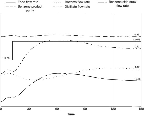
An increase in the overall volumetric flow rate of the liquid feed adds considerable liquid to the column system. Because the feed is primarily benzene, it is expected that the benzene side draw flow rate will increase. The flow rate overshoots and then assumes its new steady-state value. A similar shaped curve exists for the distillate. This is expected due to the ratio control between the distillate stream and the reflux stream and the ratio control between the benzene side draw and the reflux stream. Throughout the overshoot in flow rates, the benzene purity in the side draw remains relatively constant. What is interesting to note is the response of the bottoms flow rate. Here, an inverse response is exhibited. The flow rate first decreases, then increases, overshoots and finally assumes its new steady-state value. Why does the bottoms flow rate behave in such a manner? The introduction of more liquid feed means that more liquid benzene is cascading down the trays. As liquid reaches the bottom tray, the bubble point of the liquid on that tray decreases. The temperature controller reduces the valve opening on the bottoms stream to compensate. The reboiler level rises resulting in more steam being introduced by the action of the level controller. The benzene and pentane are vaporized and move back up the column. As the column adjusts to the increased feed flow rate, the temperature profile in the column rises. The bottoms flow rate is then increased and settles back down to its new steady-state value.
To test the control structure against changes in the composition of the feed stream, sinusoidal disturbances were introduced to the feed compositional flow rates. Each compositional flow rate was varied ±10% over periods ranging from 20 to 30 minutes. This example of a disturbance is a little unrealistic, but it demonstrates how the control structure would respond to compositional upsets. The strip chart of the same four flow rates and the benzene side draw purity is shown in Figure 8.13.
Figure 8.13 System response to sinusoidal disturbances in the component flow rates.

Each of the product flow rates responded in a similar fashion to that for a step change in the feed volumetric flow rate. As the feed flow rate increased, the products increased as well. The inverse response in the bottoms flow rate is not as observable now. The variable of interest is the benzene purity on the side draw. Although the feed composition is varying continuously, the variance in the benzene purity is much less. The affect on the benzene purity for drifting compositions is considerably damped.
8.7 Distillation Control Scheme Design Using Steady-State Models
Steady-state simulation of distillation columns has become routine. The use of these simulations has been restricted to use for heat and material balance and sizing purposes. Fruehauf and Mahoney [11, 14, 15] have shown that steady-state calculations [16] can be used to screen candidate control schemes, to provide a means for tray temperature location, and to calculate static gains.
Steady-state models are easily manipulated and are robust. This allows for the efficient generation of a large number of case studies necessary for steady-state design procedures. The obvious disadvantage of this procedure is that nothing is known about the dynamic response, and hence the dynamic disturbance rejection capability of alternative control schemes is also not known. These need to be evaluated using a dynamic simulator.
The basic steady-state design procedure consists of the following five steps:
Figure 8.14 Direct feed split control scheme.

Figure 8.15 Indirect feed split control scheme.

A case study that demonstrates the application of this design scheme is available in the literature [17].
8.7.1 Screening Control Strategies via Steady-State Simulation
Steady-state simulation can often be used to evaluate options for base level process control strategies early in the design. The advantages of such an approach are many:
For example, Shell Canada has used this approach in three recent grass-roots engineering projects and has found it to be very effective (B.J. Cott, Private communication, 2 January 2003). The following steps summarize the approach:
The approach yields a steady-state control strategy design that is optimized for the particular economics and disturbance structures used, explicitly trading off a reduced engineering cost against a potential drop in operational flexibility.
8.7.2 A Case Study – The Workshop Stabilizer
The approach is best demonstrated with an example. Here, we will examine potential control strategies for the stabilizer column described in Workshop Exercise 7. The stabilizer is designed to remove volatile components from potential gasoline blend stocks. The feed is usually a mixture of C3, C4 and C5. In this case, the feed contains 5% propane, 40% isobutane, 40% n-butane and 15% isopentane. The total flow rate is 40,000 bbl/day at 720 kPa and 30°C.
The stabilizer contains 20 trays and a total condenser. Feed enters at tray 10. The normal column overhead pressure is 700 kPa and there is a 20 kPa pressure difference that is evenly distributed between the condenser and the reboiler. Each tray is 2.0 m in diameter with a 0.10 m weir, which is 1.6 m long.
8.7.3 Respecifying Simulation Specifications
Figure 8.16 shows the column specifications in the VMGSim Simulation file as received from the process design engineer. Note that the designer has included several potential specifications for the column, of which only two can be active at any given time. Not shown are extra draw specs that can be specified on other windows within VMGSim. Here, the component fraction C3 in the bottoms and the tray 20 temperature are currently active.
Figure 8.16 Typical column specifications in VMGSim from process design (With permission from Virtual Materials Group Inc.).

A review of the potential specifications is warranted at this point. The goal is to remove any specifications that do not map onto typical instrumentation measurements. For example, flow meters work in volume units and not in molar units. Because the specifications of reflux, distillate and bottoms product rate given in Figure 8.16 are all molar flow specifications, they should not be used as control objectives. The reflux ratio and component recovery specifications are also expressed in molar units respectively and therefore cannot be used. In fact, the only specifications that can be used directly from the design simulation are
At this point, the control engineer may choose to add additional specifications to mimic other control loops. In this example, adding a specification setting the volumetric flow rate of reflux (in m3/h) would allow the control engineer to specify the reflux flow rate.
Figure 8.17 shows the column specification page with the unrealistic column specifications removed and the specifications reassigned to simulate a control strategy where the tray 20 temperature and the reflux volumetric flow are controlled. The simulation converges quickly with these two specifications active, indicating that the two control objectives are relatively decoupled.
Figure 8.17 Column respecified to simulate one potential control strategy (With permission from Virtual Materials Group Inc.).

Identifying conflicting specifications is relatively straightforward, as the simulation will take a long time to converge if conflicting specifications are used. Figure 8.18 shows that simultaneously specifying two tray temperatures result in convergence problems for the simulation. Therefore, this control structure should not be used.
Figure 8.18 Example of conflicting specifications (With permission from Virtual Materials Group Inc.).

The steady-state simulation is now prepared for control work. For simplicity, only two control strategies for the stabilizer will be investigated in this study:
Our goal is to determine which of two strategies is preferred.
8.7.4 Mimicking the Behaviour of Analysers or Lab Analyses
The process designers used the component fraction C3 in the bottoms to design the stabilizer. While it is possible to add a C3 analyser to the bottoms stream and control the C3 content to a desired value, it is more likely that the stabilizer will be run to a bottoms stream vapour pressure target, indicating the amount of light material in the bottoms stream. The Reid vapour pressure (RVP) or total vapour pressure (TVP) is a key blending property for gasoline and is typically measured via laboratory analysis.
For this work, the RVP/TVP add-in functionality from VMG (RVP Methods Extension to the Special Properties Unit Operation) was used to create a TVP measurement for the stabilizer bottoms stream.
8.7.5 Developing an Economic Profitability Function
The most straightforward means of evaluating control strategies using the steady-state simulation approach is via an economic profitability function. Working in profit makes assessment of the trade-offs between various control objectives much easier. Typically, the profitability function is given as
(8.7) ![]()
For this work, the main economic driver is maximizing the production of the bottoms stream, which will be valued at regular gasoline prices. The value of the distillate product is significantly less than that the bottoms given that its final destination is refinery fuel gas. The base value of the bottoms stream is $58.22/m3 at a TVP of 347.1 kPa. The base value of the distillate stream is $50.00/m3. Therefore, making more bottoms material at the same TVP will increase the profitability of the operation.
Because changing the volume of the bottoms product will affect its vapour pressure, the profitability function must include an adjustment for changing the bottoms product vapour pressure. The correction for changing vapour pressure is $0.25/m3/psi TVP. Therefore, if the TVP of the bottoms stream increases, the profitability of the operation will drop as this will reduce the amount of inexpensive light components that can be added to the gasoline blend and keep it on the blend vapour pressure constraint.
The value of the feed stream is $53.00/m3.
Finally, the operating costs must be accounted for. For the stabilizer column, the main operating cost is the cost of steam to reboil the column which is given as $5.6×10⁻⁶/kJ/h.
Computing the change in profitability from the base case operation is the most straightforward way of using the profitability function.
8.7.6 Evaluating the Candidate Strategies
The first step is to screen the profitability of both control strategies across a range of controller set points. Because both candidate strategies include the tray 20 temperature as a specification, it makes sense to screen it first.
Figure 8.19 shows several interesting results:
Figure 8.19 Delta profitability curves for candidate control strategies.

8.7.7 Evaluating the Candidate Strategies under Disturbances
While the behaviour of the candidate strategies appears similar to this point, it is important to examine their behaviour in relation to disturbances. To begin, the simulation was respecified to produce 200 m3/h of bottoms product since this point was found to be the most profitable operating point. Then the main disturbance was introduced: a change in the feed composition to 5% propane, 41% isobutane, 40% n-butane and 14% isopentane. Remember that the base case feed was 5% propane, 40% isobutane, 40% n-butane and 15% isopentane. The profitability of the operation was then evaluated for both strategies.
In this case, there was a large difference in the profitability. The constant reboiler duty strategy produced 187.3 m3/h of bottoms product (a drop of $18,000/day in profitability) while the constant reflux flow strategy only produced 183.3 m3/h for the same disturbance (a drop of 26,500$/day in profitability). Therefore, the constant reboiler strategy is preferred.
Typically, a wide range of disturbances would be simulated and the control performance evaluated over this range. When constructing these additional case studies, the control engineer should be aware that specific variables used as disturbances might in fact be correlated with each other. For example, the process feed rate and composition to a reactor effluent distillation process may in reality be correlated with each other because the feed rate affects the reaction kinetics via a space velocity relationship. Whenever possible, using real process data to determine the disturbance cases is preferred.
Therefore, our screening methodology indicates that, for our specific economics and specific disturbances, the constant reboiler duty strategy is preferred since its profitability is less sensitive to disturbances.
8.7.8 Evaluating Sensor Strategies
In both strategies evaluated so far, the tray 20 temperature has been standing in for the TVP analysis. Another question could be asked: What is the economic driver to do the TVP analysis online and have the control strategy directly control it? In this case, we take each disturbance case and redo the simulation specifications to control this new measurement. Then the difference in profitability between the strategies without and with the new measurement would be computed.
In our example, the tray 20 temperature control objective would be replaced with the TVP objective. For the feed composition change, the profitability of the tray 20 temperature objective is $12,6729/day while the profitability of the TVP objective is $12,8611/day. Therefore, this indicates that, for this disturbance, there is a positive economic driver to control the TVP directly of about $1880/day. Performing this same type of analysis around the range of potential disturbances and weighting the benefits as per the likelihood of the disturbance occurring, we can determine a benefit number for the analyser installation. Of course, this benefit must be balanced against the installation and maintenance cost of the TVP analyser.
8.7.9 Example Summary
The stabilizer case study has demonstrated how the effects of different control strategies on the profitability of a given process can be generated directly from steady-state simulations. The methodology requires the following:
It is these two parts that take the most time to develop when using the methodology; the actual simulation runs are only a small part of the work.
8.8 Distillation Control Scheme Design Using Dynamic Models
As detailed above, the steady-state methodology can be used to screen a large number of candidate control schemes quickly and efficiently. However, it is desirable to then evaluate the candidate control schemes using a dynamic simulator to check the dynamic disturbance rejection capabilities of the alternative control schemes. A case study that demonstrates the application of this design scheme is available in the literature [17].
The basic dynamic design procedure consists of the following five steps (which follow upon the steady-state procedure):
Table 8.1 Typical equipment hold-up times.
| Equipment | Hold-up Time |
| Heat exchangers | 30 s |
| Distillation column trays | 15–30 s (larger for crude columns) |
| Distillation column reflux accumulators | 5–10 min |
| Distillation column reboilers | 15–20 min (large enough to hold up liquid from trays, i.e. if dumped) |
| Surge vessels | 5–15 min |
A case study that demonstrates the application of this design scheme is available in the literature [17].
References
1. Buckley, P.S., Luyben, W.L. and Shunta, J.P. (1985) Design of Distillation Control Systems, Instrument Society of America, Research Triangle Park, NC.
2. Buckley, P.S. (1964) Techniques of Process Control, John Wiley & Sons, New York.
3. King, C.J. (1980) Separation Processes, 2nd edn, McGraw-Hill, New York.
4. Tyreus, B.D. (1992) Selection of controller structure, in Practical Distillation Control (ed. W.L. Luyben), Van Nostrand Reinhold, pp. 178–191.
5. Seborg, D.E., Edgar, T.F. and Mellichamp, D.A. (1989) Process Dynamics and Control, John Wiley & Sons, New York.
6. Shinskey, F.G. (1977) Distillation Control for Productivity and Energy Conservation, McGraw-Hill, New York.
7. Smith, C.A. and Corripio, A.B. (1997) Principles and Practice of Automatic Process Control, 2nd edn, John Wiley & Sons, New York.
8. Svrcek, W.Y. and Morris, C.G. (1981) Dynamic simulation of multi-component distillation. Canadian Journal of Chemical Engineering, 59(3), 382–387.
9. Wilson, H.W. and Svrcek, W.Y. (1971) Development of a column control scheme: case history. Chemical Engineering Progress, 67(2), 45.
10. Sloley, A.W. (2001) Effectively control column pressure. Chemical Engineering Progress, 97(1), 38–48.
11. Fruehauf, P.S. and Mahoney, D.P. (1994) Improve distillation-column control design. Chemical Engineering Progress, Mar, 75–83.
12. Tanaka, H., Ohara, T., Ryu, D. and Hopkins, C. (2010) Rapid analysis of gas & liquid phase using NR800 near-infrared analyzer - application to petrochemical process such as ethylene plant and chemical process. Yokogawa Technical Report English Edition, 53(2), 55–58.
13. Trevedi, Y. (1993) Controlling distillation with the most sensitive tray. Chemical Engineering, 100(1), 141–145.
14. Fruehauf, P.S. and Mahoney, D.P. (1992) Distillation column control and design using steady state models: usefulness and limitations. ISA Transactions, 32(2), 157–175.
15. Mahoney, D.P. and Fruehauf, P.S. (1994) An integrated approach for distillation column control design using steady state and dynamic simulation. Proceedings of the 73rd GPA Annual Convention, New Orleans, 7–9 March, pp. 72–80.
16. Tolliver, T.L. and McCune, L.C. (1978) Distillation column control design based on steady state simulation. ISA Transactions, 17(3), 3–10.
17. Young, B.R. and Svrcek, W.Y. (1996) The application of steady state and dynamic simulation for process control design of a distillation column with a side stripper. Proceedings of Chemeca ‘96, 24th Australian and New Zealand Chemical Engineering Conference, Sydney, The Institution of Engineers, Australia, September 1996, vol. 2, pp. 145–150.
1 Shorter natural period.