
9
Using Steady-State Methods in a Multi-loop Control Scheme
Control scheme selection for a unit operation, a process or a total plant is straightforward provided each controlled variable is only affected by one manipulated variable. However, interactions are often present between the various control loops in multi-loop control schemes. Interactions occur when a manipulated variable affects a controlled variable of another loop. For instance, in a distillation column a manipulated variable, such as reflux flow rate, may affect several different controlled variables, such as distillate flow rate, distillate composition and/or reboiler duty. Hence, selecting the best control scheme for pairing manipulated and controlled variables is not straightforward. This chapter explores different methods for designing multi-input/multi-output control schemes for processes using steady-state methods such as relative gain array (RGA), the Niederlinski index (NI) and singular value decomposition (SVD).
9.1 Variable Pairing
When multiple, single-loop control schemes interact, the closure of one loop can change the closed loop gain of one or all the other control loops in the scheme. The SISO control loops may become unstable or respond sluggishly to disturbances since the overall loop gain has been altered (Equation 2.6). The interaction between two control loops, in block diagram form, is illustrated in Figure 9.1 and is described mathematically as follows:
(9.1) ![]()
(9.2) ![]()
where yi is the controlled or output variable ‘i’, mj is the manipulated or input variable ‘j’ and aij is the input/output relationship or transfer function between yi and mj.
Figure 9.1 Loop interactions for a 2×2 system.

Figure 9.1 shows how a change in m1 will affect both y1 and y2. For a 2×2 interacting system such as this one, there are two possible control configurations. One could pair m1 with y1 and m2 with y2, or m1 could be paired with y2 and m2 with y1. The best control scheme is the one that has minimal interaction between the two control loops and will remain stable in dynamic situations, rejecting load changes or random disturbances. For a control system containing n different controlled variables and n different manipulated variables, there are n! control configurations possible. The RGA, first introduced by Bristol [1] in 1966, offers a quantitative approach to the analysis of the interactions present between the required control loops, thus providing a method of pairing manipulated and controlled variables.
9.2 The Relative Gain Array
The RGA provides engineers a quantitative comparison of how one control loop will affect others. Since it compares the effect of a manipulated variable on one controlled variable at a time, the problem is broken into more manageable segments. The disadvantage of the RGA method lies in the fact that it provides no information on the controller stability in dynamic situations, that is, during process disturbances.
9.2.1 Calculating the RGA with Experiments
Let us now consider m1 as a candidate input to pair with y1. To evaluate this choice against the alternative of using m2, the system must undergo two experiments.
Experiment 1: Step Change in m1 with All Loops Open
First, we will test the direct influence of m1 on y1. With no feedback control to affect m1 (loop 1 is open) and m2 held constant (loop 2 is open), the response of y1 can be solely attributed to the change introduced in m1. When a step change is made in m1 with all the loops open, the output y1 will change. As can be seen in Figure 9.1, y2 will also change but we will only be monitoring the response of y1. The change in steady-state value of y1 is equivalent to the steady-state gain between y1 and m1, as shown in Equation 9.3.
Experiment 2: Step Change in m1 with Loop 1 Open
Now, loop 2 is closed and the same step change is made in m1. Perfect control is assumed in loop 2, meaning that m2 will change in order to keep the controlled variable y2 at a constant value. Mathematically:
(9.4) ![]()
Since Figure 9.1 shows m1 interacting with y2 via the a21 element, m2 has to change to keep y2 constant. Changing m2 has an effect on y1 via the a12 element, and it is this interaction that is being observed.
Using the Results of Experiments 1 and 2
The relative gain is a ratio or comparison of the gain of the (mj−yi) loop with all loops open to the gain of the (mj−yi) loop with all other loops closed and in perfect control (no offset of other loop-controlled variables):
(9.5) 
The RGA or the Bristol array takes into account the relative gains for all combinations of input/output pairs in a multi-loop SISO system so that
(9.6) 
This experimental method can be repeated using m2 to control y1. Experiments 1 and 2 must be repeated, where m2 undergoes the step change and the changes in y1 are observed. For experiment 2, m1 will have to change to hold y2 at a constant value, maintaining perfect control, while m2 is subjected to its step change.
9.2.2 Calculating the RGA Using the Steady-State Gain Matrix
It is possible to calculate the RGA as previously described by performing experiments 1 and 2 on each control pairing possibility. However, this may not be feasible for an operating plant. An alternative method for calculation of the RGA is feasible if a process model is available. The process model can be used to calculate the steady-state (n×n) gain matrix, which can then be used to calculate the RGA.
The steady-state gain matrix can be calculated if one assumes that the steady-state condition is linear around each of the manipulated variables. It is a calculation that shows how each of the manipulated variables contributes to the overall effect on the controlled variables at steady state. It is also referred to as the ‘open loop gain matrix’.
Process model is available: The steady-state gain matrix, ![]() , of the process can be derived based on the process model. The steady-state gain matrix is defined as follows:
, of the process can be derived based on the process model. The steady-state gain matrix is defined as follows:
where ![]() is the vector of output or controlled variables,
is the vector of output or controlled variables, ![]() is the vector of the input or manipulated variables and
is the vector of the input or manipulated variables and ![]() is the steady-state gain or open loop matrix of the process.
is the steady-state gain or open loop matrix of the process.
Therefore, if n = 3, the steady-state gain matrix would be derived by first holding m2 and m3 constant while taking the partial derivative of y1 with respect to m1 to calculate g11, the partial derivative of y2 with m1 to calculate g21 and the partial derivative of y3 with m1 to calculate g31; then for m2 one would hold m1 and m3 constant while taking the partial derivative of y1 with respect to m2 resulting in g21 and so on.
Let the steady-state gain matrix of the process be defined as follows:
(9.8) 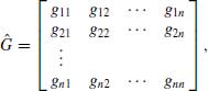
where gij has been defined in Equation 9.3 as
![]()
Now, let ![]() be the transpose of the inverse of the steady-state gain matrix,
be the transpose of the inverse of the steady-state gain matrix, ![]() , that is,
, that is,
(9.9) ![]()
The elements of the RGA can be obtained as follows:
It is important to note that Equation 9.10 indicates an element by element multiplication of the corresponding elements of the two matrices ![]() and
and ![]() . This type of multiplication is called the Hadamard product of two matrices [2], and is not the normal matrix product.
. This type of multiplication is called the Hadamard product of two matrices [2], and is not the normal matrix product.
Process model is not available: If there are no process model equations to be differentiated to obtain gij, one can use experimental results to calculate the steady-state gain matrix. Refer to experiment 1 of the RGA calculation (Section 9.2.1), where, as in Equation 9.3,
![]()
Once the steady-state gain matrix is known it can be manipulated to generate the RGA as described previously.
9.2.3 Interpreting the RGA
The RGA is a useful tool if its properties and limitations are recognized. To understand the significance of the RGA the following points should be understood [3]:
(9.11) ![]()
RGA Pairing Rules
There are some basic rules that should be followed to obtain optimal pairing in control loops:
9.3 Niederlinski Index [6]
The NI is a useful tool to analyse the stability of the control loop pairings determined using the relative gain analysis. If a manipulated variable is to be used to control an output variable, the loop must not become unstable in dynamic situations. The NI can be used to prove that a 2×2 matrix is stable; however, when n > 2 (if there are more than two input–output variables being paired) the NI can only be used to prove that the control loop is definitely not stable. Then for the steady-state matrix described in Equation 9.7:
![]()
where each element in ![]() is rational and open loop stable [3]; the system will definitely be unstable if the NI is negative, that is, if
is rational and open loop stable [3]; the system will definitely be unstable if the NI is negative, that is, if
(9.12) 
is negative.
The NI will detect instability introduced by closing the other control loops. Remember that the NI does not prove the control system is stable when there are n > 2 variables; a negative NI only proves that the system is definitely not stable.
The NI should not be used for systems with time delays (dead time). Grosididier [4] provides a detailed explanation on how to use the index for systems containing dead time. Dynamic simulation should always be used to test the stability of a system if the NI is positive.
9.4 Decoupling Control Loops
In some process situations, one manipulated variable may dominate more than one controlled variable's response. This situation is best avoided, since it is almost impossible to control such interactions. There are practical ways of dealing with such significant controller interactions and include restructuring the pairing of variables, detuning the offending control loops to minimize interactions, opening some loops (manual control) and using linear combinations of manipulated and/or controlled variables [2].
SVD [2,3] is a useful tool to determine if a system will be prone to control loop interactions resulting in sensitivity problems. These sensitivity problems typically result from small errors in process gains. This section will present and demonstrate the use of SVD.
9.4.1 Singular Value Decomposition
Ideally, manipulated variables are coupled to controlled variables on a one-to-one basis, that is, m1 controls y1, m2 controls y2 and so on, for ease of control. Since interactions do occur often between control loops, it is these controller interactions that need to be decoupled. SVD is a matrix technique useful in determining whether it is structurally impossible to apply decoupling to a system [3]. When the sets of equations in the steady-state gain matrices are nearly singular, the problem is ill-conditioned and it may not be possible to decouple control loop interactions.
SVD can be applied to the steady-state gain matrix. The gain matrix is first decomposed into the product of three matrices, where two are eigenvectors and one is an eigenvalue [2,3, 5] matrix:
(9.13) ![]()
where U is the matrix of normalized eigenvectors of GGT, V is the matrix of normalized eigenvectors of GTG and ![]() is a diagonal matrix of eigenvalues.
is a diagonal matrix of eigenvalues.
For systems where n = 2, analytical expressions have been developed to calculate the three matrices [2]. The matrix of most interest is the eigenvalue matrix ![]() .
.
For the gain matrix:
(9.14) ![]()
The following values can be defined [2]:
(9.15) ![]()
(9.16) ![]()
(9.17) ![]()
Then:
(9.18) ![]()
(9.19) ![]()
and
(9.20) ![]()
The values of s1 and s2 are always positive and the ratio of the larger si to the smaller si is called the condition number CN [2]:
(9.21) ![]()
For example, if the CN number were equal to 100, this would indicate that one manipulative variable has 100 times more effect on the system than the other manipulative variable. The higher the CN number, the more difficult it becomes to decouple a control loop interaction. A rule of thumb is when CN ![]() 50 the system is nearly singular, and decoupling is not feasible [2].
50 the system is nearly singular, and decoupling is not feasible [2].
9.5 Tuning the Controllers for Multi-loop Systems
Since a manipulated variable generally affects more than one controlled variable in a multi-loop system, it may be challenging to properly tune the system. The easiest way to work with a multi-loop system is to treat it as a group of individual control loops. First tune each loop with all the other control loops in manual. Then, close all the control loops and retune the control loops until the system can ‘handle’ a known disturbance without losing its stability. It is often necessary to loosen the original tuning parameters to minimize interactions between control loops. This entails decreasing the controller gains and increasing the integral times [3]. Dynamic simulation can then be used to drastically reduce the time required and to simplify the above controller tuning procedure.
9.6 Practical Examples
The techniques presented will now be illustrated in the following two examples, namely, a temperature control of a mixer outlet and control scheme configuration for a distillation column. The RGA will be used to select which controlled and manipulated variables will be paired, the NI will then be used to demonstrate whether or not the resulting control loops are stable and the SVD will be used to test if the control loop interactions are overly sensitive to slight errors in process gains.
9.6.1 Example 1: A Two-Stream Mixer
Consider a mixer where the hot and cold streams are being used to control the temperature and flow rate of the outlet stream (Figure 9.2). The hot stream has a constant temperature of 50°C and the cold stream has a constant temperature of 5°C. At steady state, the final desired temperature is 35°C, and the final flow rate is 600 kg/h.
Figure 9.2 Mixer control.

The equations, or process model, to describe this system are
where T is in Kelvin and the specific heat capacity of the streams are assumed constant.
At steady state the following values are maintained:
Steady-State Gain Matrix Calculation
To calculate the steady-state gain matrix, open loop gains can be found by differentiating the model with respect to mi while holding mj (j ≠ i) constant:
Equations 9.24, 9.25, 9.26 and 9.27 are open loop gains and can be evaluated by experiment 1 in Section 9.2.1 when a mathematical model is not available.
Equations 9.24, 9.25, 9.26 and 9.27 are now solved using the steady-state values listed previously. For example:
(9.28) ![]()
The steady-state gain matrix is
(9.29) ![]()
which is of the form
![]()
as described in Equation 9.7.
RGA Calculation
To calculate the RGA, first the inverse of the steady-state matrix must be found:
(9.30) 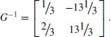
The transpose of G−1 is
(9.31) ![]()
Now, the Hadamard product of the two matrices must be calculated where ![]() . For example:
. For example:
(9.32) ![]()
So, the resulting RGA is

The RGA for this example could also be calculated by taking the ratio of the open loop gain to the closed loop gain (using the mathematical process models or experiments 1 and 2 from Section 9.2.1). For example:

![]() will now be evaluated by substituting Equation 9.22 into Equation 9.23 and solving for m1:
will now be evaluated by substituting Equation 9.22 into Equation 9.23 and solving for m1:
Substituting Equation 9.35 into Equation 9.22:
(9.36) ![]()
Now this equation must be differentiated at constant y2 and set equal to the denominator in Equation 9.34:
(9.37) ![]()
Evaluating to solve for ![]() at steady state:
at steady state:
Substituting Equation 9.38 back into Equation 9.34 to solve for ![]() results again in a value of 1/3. This result of course matches that using the ‘steady-state gain matrix’, which only required the open loop gains be calculated. This RGA shown in Equation 9.33 indicates that the best control scheme is to use m2 to control y1 and m1 to control y2. In Section 9.3, point 6 states that one should avoid pairing mj with yi when λij ≤ 0.5.
results again in a value of 1/3. This result of course matches that using the ‘steady-state gain matrix’, which only required the open loop gains be calculated. This RGA shown in Equation 9.33 indicates that the best control scheme is to use m2 to control y1 and m1 to control y2. In Section 9.3, point 6 states that one should avoid pairing mj with yi when λij ≤ 0.5.
The steady-state gain matrix for pairing y1−m2 and y2−m1 is
![]()
The resulting RGA for this y1−m2 and y2−m1 pairing is now

The rest of example 1 will be evaluated using m2 to control y1 and m1 to control y2.
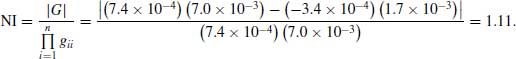
Niederlinski Index
Calculating the NI to determine whether or not the mixer control scheme will produce a stable system results in a value of 1.5 as follows:
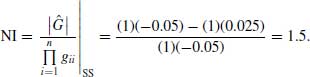
Hence, this pairing will result in a stable system, since NI > 0 and n = 2.
Singular Value Decomposition
From the RGA, it can be seen that interaction does exist between the two loops, since 0 < ![]() < 1. Whether or not this interaction will cause sensitivity problems may be determined from SVD. The SVD is calculated from the ‘
< 1. Whether or not this interaction will cause sensitivity problems may be determined from SVD. The SVD is calculated from the ‘![]() ’ as follows:
’ as follows:
![]()
where

resulting in

and
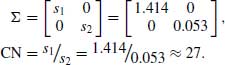
The condition number, CN, is less than 50 and, therefore, this system will not be prone to sensitivity problems [2].
9.6.2 Example 2: A Conventional Distillation Column
In this example, the RGA analysis is used to find the appropriate pairing for a conventional distillation column. There are typically two control schemes for distillation columns: single and dual composition control. The single composition control scheme maintains the composition of one of the products at a desired value, whereas in dual composition control both products are regulated.
Once the column pressure is set (typically using coolant flow rate in the condenser), the following variables can be used as manipulating variables:
The reasons why feed flow rate and reflux ratio are not considered as manipulating variables are as follows:
- The feed stream of the column is usually downstream of other units, or restated, its characteristics are usually set based on the operating condition of upstream units.
- Using reflux ratio as one of the manipulating variables results in an upset to the column whenever the distillate flow rate changes.
The variables usually considered as the process outputs for a distillation column are liquid levels at the base of the column and reflux drum and product compositions in dual composition control. Since there are four inputs that can be used to control four outputs, there are 4! different combinations. These combinations are shown in Table 9.1.
Table 9.1 Pairings in dual composition control.

A preliminary screening of these 24 alternatives based on the dynamic response of the manipulated variable to the measured variable results in the three viable alternative pairings 4, 10 and 18, which are shown in boldface in Table 9.1. The reasons for discarding other pairings are as follows:
- Schemes 1, 3, 5, 7, 9, 11, 13, 15, 19, 20, 23 and 24 are discarded since they involve control of base level by reflux flow or distillate flow.
- Schemes 6, 8, 14 and 19 are discarded since they involve manipulating the flow rate of bottom product or reboiler heat to control the liquid level in reflux drum.
- Schemes 21 and 22 are discarded since they do not regulate the material balance.
- Schemes 2, 12 and 17 are discarded since each involves the control of one (or both) product composition(s) at the end of the column using a manipulated variable at the other end of the column.
Base Case Steady-State Solution
The best pairing among these three alternatives – 4, 10 and 18 – will be found through RGA analysis of a water–ethanol distillation column. A common approach is to use a process simulation software package to determine the necessary gains for the RGA analysis and the NI. The condenser and reboiler levels will be assumed to be under perfect control. For the water–ethanol system the NRTL activity model with the ideal gas vapour model was selected. The column feed stream is shown in Table 9.2.
Table 9.2 Characteristics of the column feed.
| Conditions and Composition | |
| Temperature (°C) | 20.0 |
| Pressure (kPa) | 101.3 |
| Comp. molar flow of water (kmol/h) | 60.00 |
| Comp. molar flow of ethanol (kmol/h) | 40.00 |
The distillation column has 20 stages and a total condenser. A steady-state solution for the distillation column can be performed using the information in Tables 9.3 and 9.4.
Table 9.3 Distillation column data.

Table 9.4 Distillation column specifications for base case steady state.
| Specification | Value |
| Reflux ratio | 2.0 |
| Distillate rate (kmol/h) | 30 |
The steady-state solutions (Table 9.5) for the column yield the following results.
RGA Calculation
For this exercise, the steady-state values for the compositions will be used as the desired set points for the controllers and the best control pairings must be determined for maintaining the distillate and bottoms product compositions. The RGA will be calculated for each pairing of the three feasible alternatives: cases 4, 10 and 18 from Table 9.1.
Pairing Comparison for Cases 4, 10 and 18
At this point, the steady-state gain between the distillate flow rate and the distillate composition, g11, will be calculated using the steady-state distillation column model. Perform a step input in the distillate flow rate from 30 to 40 kmol/h. Change one of the column specifications from reflux ratio to reboiler duty, specifying a reboiler duty equal to the base case steady-state solution of 4.2×10⁶ kJ/h. The new specifications for the column should be the same as those given in Table 9.6.
Table 9.5 Base case steady-state solution.
| Mole fraction of ethanol in distillate | 0.8165 |
| Mole fraction of ethanol in bottoms | 0.2214 |
| Reboiler duty (kJ/h) | 4.2×10⁶ |
Table 9.6 Specifications for case 4 open loop.
| Specification | Value |
| Reboiler duty (kJ/h) | 4.2×10⁶ |
| Distillate rate (kmol/h) | 30 |
Run the column and determine the new mole fractions for ethanol in the distillate and bottoms. The results should be very close to those shown in Table 9.7.
Table 9.7 Steady-state solution for case 4 open loop.
| Mole fraction of ethanol in distillate | 0.7890 |
| Mole fraction of ethanol in bottoms | 0.1407 |
| Reboiler duty (kJ/h) | 4.2×10⁶ |
The open loop gain is then calculated as follows:
(9.39) ![]()
The closed loop gain, ![]() , can be calculated from the steady-state solution by closing the bottoms composition control loop, that is, making the desired bottoms composition a steady-state specification. The closed loop specifications are given in Table 9.8.
, can be calculated from the steady-state solution by closing the bottoms composition control loop, that is, making the desired bottoms composition a steady-state specification. The closed loop specifications are given in Table 9.8.
Table 9.8 Specifications for case 4 closed loop.
| Specification | Value |
| Mole fraction of ethanol in bottoms | 0.2214 |
| Distillate rate (kmol/h) | 30 |
Run the column and determine the new mole fractions for ethanol in the distillate and bottoms. The results should be very close to those shown in Table 9.9.
Table 9.9 Steady-state solution for case 4 closed loop.
| Mole fraction of ethanol in distillate | 0.6680 |
| Mole fraction of ethanol in bottoms | 0.2214 |
| Reboiler duty (kJ/h) | 2.6×10⁶ |
Now, the closed loop gain is calculated as follows:
(9.40) ![]()
At this point, the RGA matrix can be calculated because this is a 2×2 system:
(9.41) ![]()
The RGA matrix is then
(9.42) ![]()
The step changes to calculate λ11 for cases 10 and 18 are shown in Table 9.10.
Table 9.10 Open and closed loop results with the corresponding relative gain.

The resulting RGA matrix for case 10 is
![]()
and for case 18 is
![]()
Using the three RGA matrices calculated using the steady-state model of the distillation column, it can be concluded that case 10 would result in the best pairing of measured variables to manipulated variables. The RGA matrix associated with case 10 has elements that approach unity, indicating very little interaction. Case 10 uses the distillate flow rate (D) to control the top composition and the reboiler duty (QR) to control the bottom composition.
Niederlinski Index
The NI can be calculated from the full steady-state gain matrix. Using the steady-state model of the distillation column, the remaining elements for the steady-state gain matrix can be calculated for case 10. The resulting matrix is
![]()
The NI can then be calculated from
Because the NI is >0, the control pairing cannot be ruled out because it is definitely unstable. In this 2×2 case, the NI indicates that the system is stable. However, as mentioned earlier, a positive index value for higher order systems would indicate only that the system is not definitely unstable; in other words a positive index value does not indicate stability for higher order systems: the system may or may not be unstable. Therefore, one should also test the selected control scheme extensively via dynamic simulation before adoption.
Singular Value Decomposition
The SVD may now be calculated for this example from the steady-state gain matrix:

resulting in

and

The condition number, CN, is less than 50 and, therefore, this system is not prone to sensitivity problems (therefore a small error in process gain will not cause a large error in the controller's reactions) [2].
9.7 Summary
In this chapter, guidelines for pairing input and output variables in a multi-input multi-output control system have been presented using the relative gain analysis. The resulting pairings can then be tested to determine if they are definitely unstable with the NI. SVD may be used to determine if the control loops are overly sensitive to errors in process gain, as well as if the control loops may be decoupled. An in-depth discussion on these subjects is presented in the references by McAvoy [2] and Ogunnaike [3]. Dynamic simulation is a powerful tool to be used to test the viability of a control scheme during various process disturbances.
References
1. Bristol, E.H. (1966) On a new measure of interactions for multivariable process control. IEEE Transactions on Automatic Control, AC-11, 133.
2. McAvoy, T.J. (1983) Interaction Analysis: Principles and Applications, Instrument Society of America.
3. Ogunnaike, B.A. and Ray, W.H. (1994) Process Dynamics, Modeling, and Control, Oxford University Press Inc.
4. Grosididier, P., Morari, M. and Holt, R.B. (1985) Closed loop properties from steady state gain information. Industrial and Engineering Chemistry Fundamentals, 24, 221.
5. Goldberg, J. and Potter, M.C. (1998) Differential Equations – a Systems Approach, Prentice-Hall Inc., New Jersey.
6. Niederlinski, A. (1971) A heuristic approach to the design of linear multivariable interacting control systems. Automatica, 7, 691.