4

Basic Control Modes

The previous chapter discussed basic feedback control concepts including the vital role of the controller. Again, the purpose of the controller in regulatory control is to maintain the controlled variable at a predetermined set point. This is achieved by a change in the manipulated variable using a pre-programmed controller algorithm. This chapter will describe the basic control modes or algorithms used in controllers in feedback control loops.

4.1 On–Off Control

The most rudimentary form of regulatory control is on–off control. This type of control is primarily intended for use with final control elements (FCEs) that are non-throttling in nature, that is, some type of switch as opposed to a valve. An excellent example of on–off control is a home heating system. Whenever the temperature goes above the set point, the heating plant shuts off, and whenever the temperature drops below the set point, the heating plant turns on. This behaviour is shown by Equation 4.1:

(4.1)

The controller output, mv, is equal to 0% or off whenever PV exceeds the set point, SP. Whenever the process variable is below the set point, the controller output is equal to 100% or on.

The most useful type of process where on–off control can be successfully applied is a large capacitance process where tight level control is not important, that is, for the case of flow smoothing. A good example of this type of process is a surge tank. A large capacitance is important due to the nature of the controller action and its effect on the operational life of the FCE. This leads us to one of the disadvantages of an on–off type of controller. Due to the continual opening and closing of the controller, the FCE quickly becomes worn and must be replaced. This type of control action is illustrated in Figure 4.1, which shows the typical behaviour of an on–off controller.

In this example, at time t = 0, PV is less than SP, and mv is equal to 100%. When PV crosses the set point, mv becomes 0%. The temperature rises somewhat above the set point before the controller turns off because of dead time, the capacitance of the heating system and heat transfer to the ambient. These factors are termed system dynamics. When the temperature drops below the set point, the controller opens the valve. However, again due to system dynamics, the temperature drops somewhat below the set point before PV begins to rise again. It is easy to see how the FCE would quickly become worn out when this action is continually occurring.

Since the controller cannot throttle the actuator, but only turn it on or off, the primary characteristic of on–off control is that the process variable is always cycling about the set point. The rate at which PV cycles and the deviation of PV from the set point are a function of the dead time and capacitance in the system, or the system dynamics. The longer the lag time the slower the cycling, but the greater the deviation from the set point. This can better be illustrated by using an on–off controller with a differential gap or dead band as shown in Figure 4.2. Most on–off controllers are built with an adjustable differential gap or dead band, inside which no control action takes place. The intent of this differential gap is to minimize the cycling of the controller output and extend the operational life of the FCE.

The controller switches off when the process variable exits the dead band on the high side and does not turn on again until PV is outside the dead band on the low side. The frequency of cycling is reduced, but the deviation from the set point is increased. If the dead band is reduced the frequency of cycling is increased but the deviation from the set point is decreased.

Typically, the dead band is adjusted as a percentage of the process variable span. Using the heating system example, suppose the temperature measurement range was from 20° to 120°. Setting the dead band equal to 10% of the span, the dead band in degrees would be 10°. If the set point were 75°, then the upper edge of the dead band would be 75°+5° = 80° and the lower edge of the dead band would be 75° − 5° = 70°, giving the dead band a width of 80° − 70° = 10°.

With an on–off controller cycling cannot be eliminated. When a large lag is present in the process, the deviation from the set point may not be perceptible since the amount of time per cycle is longer. If this is acceptable, an on–off controller can be used. However, in order to eliminate cycling completely, another control mode would need to be implemented.

4.2 Proportional (P-Only) Control

Proportional control is the simplest continuous control mode that can damp out oscillations in the feedback control loop. This control mode normally stops the process variable, PV, from cycling but does not necessarily return it to the set point.

For example, consider the liquid level control situation given in Figure 4.3, in which the tank must not overflow or run dry. If the inflow, Fi, is equal to the outflow, Fo, then the level, as seen in the sight glass, remains constant. If Fo increases such that it is greater than Fi, the level will begin to drop. In order to stop the level from dropping Fi must be increased by opening the inflow valve until it is equal to Fo, and the level stops dropping. However, the tank level is no longer at the initial level; it has dropped to a new steady-state level. The amount the level drops depends on how much the inflow valve had to move to make Fi equal to Fo. A similar situation would occur if Fo was less than Fi, only in this case the level would rise until the readjusted inflow equals the outflow. This scenario describes what a proportional controller would do if it were connected to the tank.

In equation form the output of a proportional controller is proportional to the error1 (Equation 4.2):

(4.2)

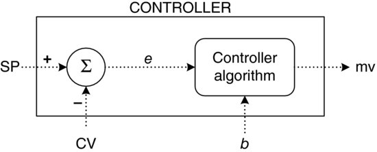
In Equation 4.2, Kc is the controller gain, e is the error and mv is the manipulated variable. Remember:

To allegorize proportional control we will use the liquid level loop shown in Figure 4.3. Initially, the proportional controller is placed in manual and the level in the tank is manually adjusted to equal the set point. With Fi equal to Fo, the level should stay at the set point. Also, set Fo = 50% = Fi, CV = SP = 50% and Kc = 2. Note that here we are using percent of span units. Now, if the controller is placed into auto what will happen to the output? At the instant the controller is placed into auto, the error will be zero since CV is equal to SP, and the controller output will also be zero:

For a controller output of zero, what will the level do? The level will begin to drop. To stop this movement Fi and Fo must equal 50% again. If a linear relationship is assumed between inflow and controller output, then for Fi = 50% we will have mv = 50%.

Thus, the controller output becomes 50% when the measurement, CV, drops by 25%, creating a 25% error. For this case, in order to stop the level from dropping, the proportional controller had to drop CV to create a large enough error so the controller could make Fi = Fo.

Suppose Kc was set equal to 4, giving mv = 4e. Now, the error would only need to be 12.5% for mv = 4(12.5%) = 50%. Logically, it would appear that the larger the controller gain, the smaller the error. In theory if Kc is set to infinity the error can be reduced to zero. The problem with this extrapolation is that the gain of the controller, Kc, is multiplied by all the gains of the other elements to give the loop gain, KL. If Kc becomes large enough, the loop gain will be greater than one, thus causing the loop to become unstable. Because of this loop gain limit, there is a limit to how large the controller gain can be. However, there is another approach to reducing the error to zero. Suppose another term was added to the proportional controller equation, as shown in Equation 4.3:

(4.3)

This additional term is called the bias, b, and is simply defined as the output of the controller when the error is zero. Using the previous example again, let us set Kc equal to 2. Also, manually adjust CV = SP = 50%, Fi = Fo = 50% and set b = 50%. Now, when the controller is set to auto, what will happen? Since CV is equal to SP, e is equal to zero and, hence, Kce = 2(0) = 0. There is no proportional contribution to the output and the output, mv, is equal to the bias which is 50% (Equation 4.3). Since Fo is equal to 50% and mv is also equal to 50%, the level will stay the same. In general, if the bias equals the load, mv, the error will always be zero.

Now, suppose Fo becomes 75%. In order to stop the level from dropping, mv must equal Fo, which in this case is 75%. From Equation 4.3, mv = 2e+50% = 2(50% – CV)+50% and CV must drop to 37.5% to make the output, mv, equal to 75%. When mv is equal to the outflow, the level will stop dropping. The level could also be prevented from dropping if the outflow, Fo, was decreased. Suppose Fo is equal to 25%. In this case, the level will stop rising when CV is equal to 62.5%, since that gives mv = 2(50% – CV)+50% = 25%.

As previously mentioned, increasing Kc can decrease the error, but remember not to increase Kc such that it makes the loop unstable. There is a limit for each feedback control loop. If Kc has a value such that the loop gain, KL, is equal to one, the loop will oscillate with a period that is a function of the natural characteristics of the process. This is called the natural period, τn. If Kc is adjusted such that the loop gain is equal to 0.5 and a change is made in Fo, the response shown in Figure 4.4 could be expected.

CV damps out with a quarter decay ratio2 and a period approximately equal to the natural period. It then stabilizes with an offset that is a function of both the controller gain and the bias. The offset is the sustained error, e, where CV does not return to the set point even when steady state is reached. This is a typical response for a loop under proportional-only control.

Now let us look again at Equation 4.3 and recall that the gain of any loop element is defined by Equation 4.4:

(4.4)

The block diagram of a proportional controller can be represented as shown in Figure 4.5.

The controller gain is the ratio of the change in controller output to the change in error. Hence, the gain of the proportional controller, Kc, is given by Equation 4.5:

(4.5)

Since there is a one-to-one relationship between CV and e the controller gain can be written as per Equation 4.6:

(4.6)

The controller gain can also be defined as a change in controller output for a change in the process variable, PV. This is true because the controlled variable, CV, is the transformed process variable from the transmitter to the controller. Therefore, CV is essentially PV, only in different units, that is, % level instead of milliamperes.

Assuming that a linear relationship exists between CV and mv, as shown in Figure 4.6, Equation 4.7 may be written as follows:

(4.7)

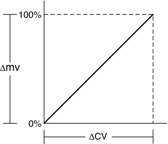
The controller gain, Kc, in Equation 4.7, is the amount that CV must change to make the controller output change by 100%. The gain of the transmitter is similar and is given by Equation 4.8:

(4.8)

In other words, the input of the transmitter changes by the amount of the span to make the transmitter output change by 100%. The span is the difference between the upper and lower values of the range.

The case of the controller is analogous to that of the transmitter, but instead of calling ΔCV the span, it is called PB, the proportional band. The proportional band is defined as the change in CV that will cause the output of the controller to change by 100%. Using this definition of PB we can define the controller gain as shown in Equation 4.9:

(4.9)

If the proportional band setting on the controller is set to 40%, the output of the transmitter, which is the input to the controller, changes over 40% of its output span. The output of the controller would change by 100%, or the controller gain, Kc, would be

Virtually all modern controllers use a gain adjustment, however a few older controllers exist that still use a proportional band adjustment. Remember that , or as the PB gets larger, the gain gets smaller and vice versa. The equation for a proportional controller in terms of PB can be written as follows:

(4.10)

Note that

In order to make the error equal to zero, one of the following two possibilities must occur:

The first option, as previously discussed, is not plausible since as PB → 0, Kc → ∞ and the loop becomes unstable. Furthermore, it is not possible to set PB = 0, because on many controllers the minimum setting is usually 2–5%. However, if PB was very small, that is, 2% or Kc = 50, the error would certainly be minimized, provided the loop remained stable. This case can be illustrated using Figure 4.7.

If in Figure 4.7, , then the loop would be stable since the loop gain KL < 1 (Equation 2.6). If the process had a lower gain, KP, then a higher controller gain or smaller PB in the P-only controller could be used to minimize the error. One type of process where this is the case is a very large capacitance process, that is, a large surge tank. Due to the low process gain, a P-only controller is often used for level control.

The second option to make the error zero is to set the bias equal to the controller output, mv. Some controllers have an adjustable bias and hence make this option viable, as in Equation 4.11:

(4.11)

However, this approach is only an option for processes that experience few load upsets, since a manual readjustment of the bias is required each time there is a load upset. There would be no error as long as the bias was equal to the load. Hence, if the process had infrequent load upsets, the operators could readjust the bias to give zero error, and it would be possible to use a P-only controller.

In general, a proportional controller provides a fast response when compared to other controllers but a sustained error occurs where the PV does not return to the set point even when steady state is reached. This sustained error is called offset and is undesirable in most cases. Therefore, it is necessary to eliminate offset by combining proportional control with one of the other basic control modes.

4.3 Integral (I-Only) Control

The action of integral control is to remove any error that may exist. As long as there is an error present, the output of this control mode continues to move the FCE in a direction to eliminate the error. The equation for integral control is given as

(4.12)

mvo is defined as either the controller output before integration, the initial condition at time zero or the condition when the controller is switched into automatic. The block diagram for an integral-only controller is given in Figure 4.8.

The action or response of the integral control algorithm for a given error is shown in Figure 4.9, assuming increase/decrease action.

If the measurement, CV, was increased in a stepwise fashion at time t1 and then returned to the set point at t2, the output would ramp up over the interval t1 < t < t2 since the controller is in effect integrating the step input. When the measurement is returned to the set point at t = t2, the output would hold the value that the controller had integrated to, since the controller would think this was the correct value or the set point, that is, e = 0.

The rate at which the controller output ramps is a function of two parameters: the integral time, Ti, and the magnitude of the error. Obviously, the controller output, mv, would ramp in the opposite direction if CV had been moved below the set point.

The integral time, Ti, is defined as the amount of time it takes the controller output to change by an amount equal to the error. In other words, it is the amount of time required to duplicate the error. Thus Ti is measured in minutes per repeat. Because of the form of Equation 4.12 some manufacturers measure the reciprocal of Ti or repeats per minute in a controller (Equation 4.13):

(4.13)

As a result of this reciprocal relationship, if the controller is adjustable in min/rep, then increasing the adjustment gives less integral action, whereas in rep/min, increasing the number produces greater integral action. Therefore, it is important to be aware of how an individual controller adjusts Ti. The rate of change of mv also depends on the magnitude of e as shown in Figure 4.10, in which Ti is fixed.

Figure 4.11 illustrates the responses of P-only, I-only and PI controllers to a step input. Although an integral-only controller provides the advantage of eliminating offset, there is a significant difference in its response time when compared to proportional-only controller. As mentioned earlier, the output of the proportional-only controller changes as quickly as the measurement changes; in other words, the controller tracks the error. So, if the measurement changes as a step, the controller output also changes as a step by an amount depending on the controller gain. For a step input to an integral controller, the output does not change instantaneously but rather by a rate that is affected by Ti and e.

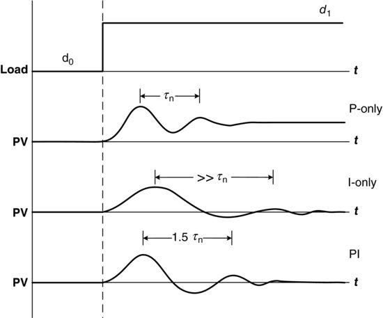
Hence, integral-only control, due to the additional lag introduced by this mode, has an overall response that is much slower than that for proportional-only control. The period of response for the PV under integral-only control can be up to 10 times than that for proportional only; so a trade off is made when using an I-only controller. If no offset is required then a slower period of response must be tolerated. If the requirement is a return to the set point with no offset, and a faster response time is necessary, then the controller must be composed of both proportional and integral action.

As a result of the above, controllers with both proportional and integral action are more common. However, a few examples of integral-only controllers do occur. In the Claus sulfur plant air demand controller [1] the trim air valve position error may be used to drive the main air valve position using only integral action. The combination of small (trim) and large (main) valves permits fine control of the Claus sulfur plant furnace air demand. In energy or ‘BTU’ control of a coal-fired power station (L. Neumeister, Personal Communication) the integral-only control compares the energy leaving the boiler (steam) with the energy entering the boiler (coal). If there is a sustained difference, the integral-only controller modifies the energy content of the coal feed until there is an energy balance. The integral time is very small and is intended to compensate for the energy content of the supplied coal. Typically it takes some 12 hours for the BTU content of the coal to change a significant amount.

4.4 Proportional Plus Integral (PI) Control

A proportional plus integral controller will give a response period that is longer than a P-only controller but much shorter than an I-only controller. Typically, the response period of the process variable, PV, under PI control is approximately 50% longer than for the P-only (1.5τn, Figure 4.11). Since this response is much faster than I-only, and only somewhat longer than P-only control, the majority (>90%) of controllers found in plants are PI controllers. The equation for a PI controller is given in Equation 4.14:

(4.14)

The PI controller gain has an effect not only on the error, but also on the integral action. When we compare the equation for a PI controller (Equation 4.14) to that for a P-only controller (Equation 4.11) we see that the bias term in the P-only controller has been replaced by the integral term in the PI controller. Thus, the bias term for PI control is given by Equation 4.15:

(4.15)

Therefore, the integral action provides a bias that is automatically adjusted to eliminate any error. The PI controller is faster in response than the I-only controller because of the addition of the proportional action, as illustrated in Figure 4.12.

As shown in Figure 4.9, it takes Ti minutes for the output of the I-only controller to duplicate the error. With the addition of proportional action there is an immediate proportional step followed by integral action. The integral time in this case is defined as the amount of time it takes for the integral portion of the controller to replicate the proportional action. When the measurement is returned to the set point, the proportional action is lost since e = 0, and the controller output is determined solely by integral action.

As can be seen from Equation 4.16, the gain of the PI controller, KPI, is the sum of the two component gains. These component gains are proportional action, KP, and integral action, KI:

(4.16)

The Kc and Ti are used to adjust the PI controller gain to give the loop a desired response. Suppose Ti = ∞, which would result in KI = 0, regardless of the value of Kc. In effect, the response would be that of a P-only controller with a period equal to τn and a sustained error. While Ti = ∞ is not realizable, it can be set to a very large number in min/rep to minimize the integral action.

Now, suppose Ti were set to a very small value. In this case, the PI controller gain would approach that of an integral-only controller, since KI >> KP. The control action in the loop would now be that of an I-only controller with a return to the set point but a long response period.

These are two extremes and somewhere in between is a Ti that will give a return to the set point with a reasonable response period of 1.5τn. The selection of Ti will be discussed in more detail under controller tuning in Chapter 5.

In general, starting with only proportional action, as more integral action is added, the PV begins to return to the set point. We only want enough integral gain to return to the set point, since a KI greater than this will only serve to lengthen the response period. As more integral action is added by reducing Ti, we must compensate for the increased integral gain by reducing the proportional gain. Adjusting Ti will have an effect on KI and thus affects KPI, which in turn affects both the damping and the response period. Adjusting Kc affects both KI and KP equally, thus Kc only has an effect on KPI, affecting the damping and not the response period. These interacting effects will be considered in more detail under controller tuning in Chapter 5.

Although the response period of a loop under PI control is only 50% longer than that for a loop under P-only control, this may in fact be far too long if τn is as large as 3 or 4 hours. In order to increase the speed of the response it may be necessary to add an additional control mode.

4.5 Derivative Action

The purpose of derivative action is to provide lead to overcome lags in the loop. In other words, it anticipates where the process is going by looking at the rate of change of error, de/dt. For derivative action, the output equals the derivative time, Td, multiplied by the derivative of the input, which is the rate of change of error (see Equation 4.17):

(4.17)

Figure 4.13 shows how the output from a derivative block would vary for different inputs given a fixed value of Td.

As the rate of change of the input gets larger, the output gets larger. Since the slope of each of these input signals is constant, the output for each of these rate inputs will also be constant. However, what happens as the slope approaches infinity as in the case of a step change, (4) in Figure 4.13? Theoretically the output should be a pulse that is of infinite amplitude and zero time long. This output is unrealizable since a perfect step with zero rise time is physically impossible, but signals that have short rise and fall times do occur. These types of signals are referred to as noise. Thus, the output from the derivative block would be a series of positive and negative pulses, which would try to drive the FCE either full open or full close. This would result in accelerated wear on the FCE and no useful control.

Consider a temperature measurement with a small amplitude and high-frequency noise. One might assume that since the noise is of such small amplitude in comparison to the average temperature signal, a controller would not even notice it. This is only the case if the controller does not have derivative action. If the controller contains derivative action, the temperature signal would be completely masked by the noise into the derivative mode of the controller, and the controller output would be a series of large amplitude pulses, entirely masking any output contributed by the other control modes. Fortunately, in a case such as this the noise is either easily filtered out or eliminated by modifying the installation of the primary sensor.

However, there are cases where noise is inherent in the measurement of PV and the rise and fall times of the noise is of the same magnitude as that of the measurement itself. In such a case, noise filtering would only serve to degrade the accuracy of the measurement of PV. A good example of a situation like this is a flow control loop. Flow measurement by its very nature is noisy and therefore, derivative action cannot be successfully applied.

It is important to note that derivative control would never be the sole control mode used in a controller. The derivative action does not know what the set point actually is and hence cannot control a desired set point. Derivative action only knows that the error is changing.

4.6 Proportional Plus Derivative (PD) Controller

The minimum controller configuration containing derivative action is the combination of proportional plus derivative action shown in Equation 4.18. This combination is not used very often and is primarily applied in batch pH control loops. However, it will help in the definition of derivative time, Td:

(4.18)

In Equation 4.18, the PD controller equation contains a bias term. A bias term will normally appear in any controller algorithm that does not contain integral action. This bias term does not appear when integral action is present since integral action is in effect an automatic adjustment of bias. As with the PI controller, the proportional gain acts on the error as well as the derivative time, Td. Figure 4.14 shows the controller output (mv), for a typical input (e) test signal for the proportional and derivative portions of a PD controller.

In Figure 4.14, mvP is the proportional portion of the output and mvD is the derivative portion. In the example, the measurement changes at a fixed rate of change, and therefore, the derivative portion of the output is constant and depends on the rate of change, the derivative time, Td, and proportional gain (Kc). This dependency is evident from Equation 4.18. The proportional output is a ramp whose slope is a function of the proportional controller gain, Kc.

Now, let us superimpose mvP and mvD to get the actual output for a PD controller, shown in Figure 4.15.

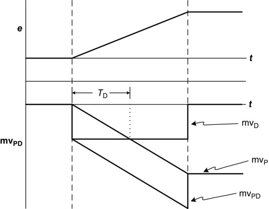
For a ramp input it takes a period of time for the proportional action to reach the same level as the derivative action. This period of time is called the derivative time, Td, and is measured in minutes. Increasing the derivative time, Td, increases mvD, or the contribution of the derivative action to the movement of the final control element.

In Equation 4.18, for the PD controller the derivative action acts on the error. Since e = SP – CV for I/D action, de/dt is a function of both the derivative of the set point, dSP/dt, and the derivative of the controlled variable, dCV/dt (Equation 4.19):

(4.19)

If there is a load upset to the process, the process variable, PV, will change at some rate, dCV/dt which will result in the error also changing at the same rate (de/dt = −dCV/dt), assuming there is no set point change. Now, if a set point change of even a few percent is made and if the set point is changed quickly, then dSP/dt can become very large. This would cause a large pulse to be generated at the output of the controller. To overcome this potential problem, the controller can be made so that the derivative mode simply ignores set point changes as shown in Equations 4.20, 4.21 and 4.22:

(4.20)

Ignoring set point changes gives

(4.21)

Hence,

(4.22)

In other words, there is no derivative action on a set point change, only proportional action. On a load upset both proportional and derivative actions are enabled. (Note also that in some controller implementations, the proportional action is also decoupled from set point changes as the kick from a set point change is also considered to be too aggressive).

Figure 4.16 shows a comparison of the control loop response to a load upset for both P-only and PD control. The response of the measurement, PV, under PD control is faster and results in a smaller offset than the loop under P-only control. This faster response is due to the addition of the derivative action.

In a PI controller, in order to minimize the integral action, Ti was made a large number. This makes the integral gain approach zero, and the controller then behaves essentially like a P-only controller. However, in the PD controller, even by setting Td to a very small value, there is still the possibility of a sizeable derivative contribution if there is a noisy input, that is, if dCV/dt is large.

In electronic controllers and distributed control systems (DCSs) the derivative action can be eliminated by setting Td to zero. In a pneumatic controller the derivative action cannot be eliminated but can be reduced to a minimum value of approximately 0.01 minute. If a PD controller is installed on a flow loop there will still be considerable derivative action due to the noisy flow measurement. It is therefore important, when applying a pneumatic controller to a noisy loop such as a flow loop, to make certain the controller does not contain a derivative block.

The main reason for interest in derivative action is to combine it with proportional and integral actions to produce a three-mode controller, PID.

4.7 Proportional Integral Derivative (PID) Control

The primary purpose of a proportional integral derivative controller (see Equation 4.23) is to provide a response period, τn, that is much the same as with proportional control but which has no offset. The derivative action adds the additional response speed required to overcome the lag in the response from the integral action:

(4.23)

Figure 4.17 presents a comparison of the responses for a P-only, PI and PID controllers to a step change in load.

The addition of the derivative mode in the PID controller provides a response similar to that of a P-only controller but without the offset because of the integral action. Therefore, a PID controller provides a tight dynamic response, but since it contains a derivative block it cannot be used in any processes in which noise is anticipated.

4.8 Digital Electronic Controller Forms

Controller algorithms are implemented in digital electronics using digital or ‘discrete-time’ forms of the analog or ‘continuous-time’ controller algorithms presented above. There are two basic digital electronic controller algorithms – the positional form and the velocity or differential form.

The positional form of the PID controller algorithm is

(4.24)

where mv(t), e(t) and CV(t) are the current controller output, error and controlled variables, respectively; t is the enumerated sampling instant in time; mv(t – 1), e(t – 1) and CV(t – 1) are the values of the controller output, error and controlled variables, respectively, one sampling period ago; and h is the sampling period.

The velocity or differential form of the PID controller algorithm is

(4.25)

For the positional form it is important to note how to handle properly the summation term associated with the integral action. The integral term in Equation 4.24 could grow to become a very large value if the output device was saturated and the CV was not able to return to the set point. For situations such as this, it is important to reset the value of the summation to ensure that the output of the algorithm will be equal to the (upper or lower) limit of the controller output. Then when the set point is changed to a region where the controller can control effectively the controller will respond without having to decrease the summation term from a value that has grown way beyond the upper or lower limit of the output. This automatic resetting of the controller integral term is commonly called anti-reset windup.

The velocity or differential form does not suffer from reset windup and is therefore the preferred form of controller equation when integral action is required. However, the positional form is preferred when there is no integral term because this is the fail-safe form (in that in the advent of a failure the controller output will fail fully open or closed depending on the design) – whereas the failure mode for the velocity or differential form is the last value of the output.

4.9 Choosing the Correct Controller

Now that the various basic control modes have been described, it is desirable to be able to choose a particular control mode for a specific process. Figure 4.18 graphically outlines a procedure for control mode selection.

Starting at the top of the flow diagram, the first decision block asks the question: ‘Can offset be tolerated?’ If the answer is yes, a proportional-only controller can be used. If the answer is no, proceed to the next block which asks ‘Is there noise present?’ If there is noise, then use a PI controller. If there is no noise, proceed to the next block, which asks ‘Is dead time excessive?’ If the ratio of the dead time to the process time constant is greater than 0.5, the process can be assumed to be dead-time dominant and requires a PI controller. If the process has no excessive dead time, then the next block asks ‘Is the capacitance extremely small?’ If the answer is yes, then a PI controller can be used. A process with a short dead time and small capacitance does not require derivative action to speed up the response since it is already fast enough, as is the case for a flow loop. In this instance we might even consider an I-only controller since the loop is so fast that slowing down the response through the use of integral-only action will still provide a fast enough response for the majority of applications in the fluid-processing industries. Finally, if the process capacitance is large, a PID controller can be effectively used.

It was mentioned earlier that the PI controller is the most common controller found in the plant. Looking at this flow chart one can see why. There are three possible paths to the PI controller, while there are four decision blocks that must be passed through to reach a PID controller.

4.10 Controller Hardware

Now that we have covered how the controller works it is necessary to discuss controller hardware. Figures 4.19 and 4.20 are examples of single-loop stand-alone controllers. Figure 4.19 is an electronic analog controller, from the 1970s.

Figure 4.20 is an old version of the electronic digital controller. It contains additional functionality such as alarm limits for process value, deviation output signal and set point, set point ramping, auto or self-tuning, signal filter time constant adjustment, startup values, on/off modality and gain schedule limits. A more current DeltaV™ digital controller is shown in Figure 4.21.

Figure 4.22 shows a screenshot from a modern DCS. Simply put, a DCS is an electronic digital control system where computers spread functionality over multiple processes in large-scale plants. The advantage of a DCS is that it allows operators to monitor and control entire plants from a central control room.

DCSs were introduced in the mid-1970s with the advent of the microcomputer. DCSs enabled more flexible and complex control, monitoring, alarming and historic data trending than local, single-loop control, or the centralized control previously possible with minicomputers.

Modern DCSs feature the use of digital, multi-drop communications that can interconnect sensors, actuators and the control room. Control can be allocated to the digital devices that can communicate directly with each other to fully exploit each other's capabilities with remote diagnostics and supervisory control and data acquisition (SCADA). This control technology is known as Fieldbus (http://www.fieldbus.org/) [2]. Additional detail pertaining to Foundation Fieldbus for instrumentation and control can be found in Appendix 3 (A. Dicaire, Personal communication; B. Van Vliet, Personal communication).

With the ability to send data wirelessly, information to and from field devices can be sent and received at a single I/O point via a gateway that has coverage for up to 100 different devices. Examples are shown in Appendix 3 (B. Van Vliet, Personal communication). Back in the panel, electronic marshalling unique to DeltaV can be done too. It is based on traditional I/O practices, but delivers value in reduced infrastructure and associated engineering design [3].

The PC explosion of the 1980s and 1990s has also impacted modern DCSs with the advent of PC-based control systems [4,5] which feature object linking and embedding (OLE) software for process control (OPC) (http://www.opcfoundation.org/).

References

1. Young, B.R., Baker, J.T., Monnery, W.D. and Svrcek, W.Y. (2001) Dynamic simulation improves gas plant SRU control-scheme selection. Oil & Gas Journal, May 28, 54–57.

2. Hodson, W.R. (1998) A Fieldbus primer. Oil Patch Magazine, Nov./Dec., 7–9.

3. DeltaV I/O on Demand, http://www2.emersonprocess.com/en-US/brands/deltav/differentiators/Pages/IOonDemand.aspx (November 2011).

4. DeltaV™. (1996) Fisher Rosemount Systems, Inc., USA.

5. Santori, M. (1997) The emergence of PC technology. Chemical Engineering, Dec., 70–78.

1 Error is the deviation of the measurement, CV, from the set point, SP.

2 Quarter decay ratio is discussed in greater detail in Chapter 5.