
3
Fundamentals of Single-Input/Single-Output Systems
In this chapter, we describe the basic components and concepts of single-input/single-output (SISO) control systems, along with some of the physical attributes commonly found in these systems. We will also explain the characterization of system responses and provide an introduction to modelling various processes. After studying this chapter, the reader should understand
- the basic components of a SISO process control loop;
- the difference between open loop and closed loop control;
- the concept of direct-acting and reverse-acting controls;
- what process capacitance is and what it contributes to process controllability;
- what process dead time is and what challenges it poses to process controllability; and
- how to develop some of the basic equations that govern first-order system response with feedback control.
We recommend that the student review the fundamentals of differential equations and some of the more common numerical methods to aid in understanding the mathematical development and solution of the various process models presented in this chapter. Some excellent sources for such a review are included in the references [1–3].
3.1 Open Loop Control
Most readers will be familiar with how the speed of an automobile is controlled. The basic ‘process’ set-up is quite standard, as illustrated in Figure 3.1. There is an air/fuel mixture feed, a throttle that regulates how much feed is introduced and the engine itself that converts combustion energy into rotating mechanical energy that turns the wheels at a certain rpm. Consider a car on a straight, flat road on a still day. Move the throttle to just the right position and you will achieve the desired speed. Once set, there is no need to adjust it. After all, if nothing changes in the environment, the rpm of the engine should stay right where it is. This is a familiar example of open loop control.
Figure 3.1 Illustration of car metaphor.
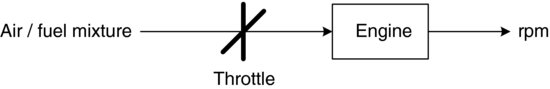
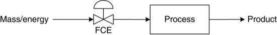
Figure 3.2 illustrates a more generic process than our automobile example, but the basic elements are the same. Here, instead of air/fuel mixture feed, we use the term mass and energy feed. Instead of a throttle, we call it a final control element (FCE). Instead of an engine, we have a process. And instead of an output rpm, we call the measured output of the process, the controlled variable/process variable.
Figure 3.2 A simplified process view.
By definition, open loop control places the FCE in a fixed position, or a prescribed series of positions, with the expectation that nothing will change (i.e. there will be no disturbances) to cause the desired state of the system (set point value) to drift. Other examples of open loop control are traffic lights and a washing machine cycle. Once the control action is initiated, it will proceed through the prescribed steps or remain fixed without any knowledge of the actual status of the process. Sometimes this actually works. Much of the time, however, it does not. Consider our automobile example, if the road is suddenly rising steeply or a strong headwind is encountered.
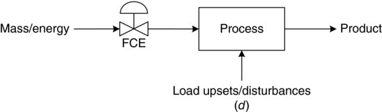
A more realistic view of a process or plant is shown in Figure 3.3.
Figure 3.3 A realistic process view.
3.2 Disturbances
The process shown in Figure 3.3 adds the more realistic dimension of upsets or disturbances, d. Upsets and disturbances typically come in three types: input disturbances, load disturbances and set point disturbances. An input disturbance is a change in the mass or energy of the supply, or input, to the process that may cause the condition of the process variable to drift from its set point value, SP. A load disturbance is any other upset, except for an input mass or energy change, which may alter the quality of the process variable from the desired set point value. A set point disturbance occurs when the desired state of the process variable (PV) changes, and the process must adjust to a new state. The biggest difference between input disturbances and load disturbances – and the reason we distinguish between them – is that load disturbances cannot typically be anticipated, and they are often not measured directly. The only way we find out about them is by observing the effect they have on the product conditions or quality. While input disturbances may also be difficult to anticipate, they are often measured, and corrective action can more readily be taken. For this reason, we will primarily focus on load disturbances for the remainder of this chapter.
Returning to our automobile example and adding the more realistic dimension of disturbances, we see that in order to ensure we keep a steady rpm, we need to be able to constantly adjust the throttle position in order to keep a constant speed. This is essentially the function that cruise control carries out and is an example of automatic feedback control. Simply put, automatic feedback control provides an automatic adjustment to the FCE in an attempt to maintain the conditions of the process variable at the desired set point value, SP, in the presence of disturbances, d.
3.3 Feedback Control – Overview
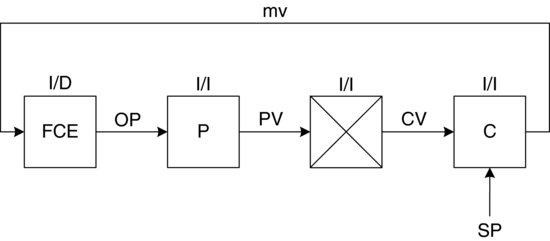
The simplest and most widely used method of process control is the feedback control loop shown in Figure 3.4. Existing control practitioners should recognize this figure is an alternative form of a classical block flow diagram (Figure 3.5) that is seen in most process control textbooks. Both Figures 3.4 and 3.5 illustrate the same things – both the information flow and physical connections of the feedback control loop. (In this book we use a format that more closely resembles instrumentation or control systems diagrams that are used in real process design documentation, e.g. P&IDs and control systems narratives).
Figure 3.4 Single-input/single-output feedback control loop.

Figure 3.5 Alternative, classical form of the single input/single output feedback control loop.
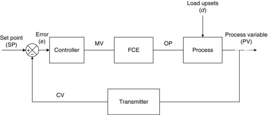
In the feedback control loop we take a measurement of the process variable (indicated by CV, or controlled variable, in Figure 3.4) we care about (Transmitter in Figure 3.4 means ‘measuring device’) and this value is compared to a set point (SP) to create an error, or departure from aim. In Figure 3.4, OP indicates the operating point around which this calculation takes place. This error is used to drive the corrective action of the FCE via the controller. Note that the output of the controller ‘manipulates’ the mass and energy into the system via the FCE. Thus, the property that the controller manipulates is referred to as the manipulated value, or mv. The action of the controller may be aggressive or sluggish; it depends on the internal equations of the controller (sometimes called the control algorithm or control law) and the tuning that is used. We will discuss controller types in Chapter 4 and tuning in Chapter 5. In order to successfully control a process, it is important to select both the right process variable and the right manipulated value. The process variable is typically a temperature, pressure, flow, composition or level and is typically a variable that (a) is important to the product quality or the process operation and (b) is responsive to changes in the selected manipulated value.
It is interesting to note that if an automatic feedback controller succeeds in keeping the PV at the desired SP in the presence of load disturbances then, by necessity, there will be changes in the mv dictated by the controller. So in effect, process control takes variability from one place, and moves it to another. Thus, the trick to process control is understanding where variability can be tolerated and where it cannot and designing schemes that manage variability to acceptable levels.
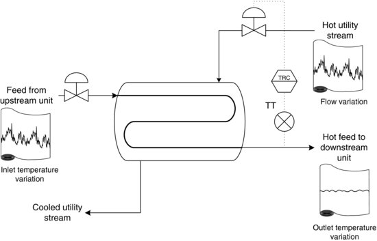
The heat exchanger, shown in Figure 3.6 [4], illustrates this transference of variability. The temperature of the ‘Hot Feed to Downstream Unit’ stream is important to control (its temperature is the PV for this controller). The ‘Hot Utility’ stream flow is manipulated (it is the mv for this controller) in order to keep the PV at its set point in the presence of load disturbances introduced in the ‘Feed from Upstream Unit’ stream. With no control, these disturbances would make their way into the ‘Hot Feed to Downstream Unit’ stream. With control, the mv absorbs these disturbances while keeping the PV at or near the set point. Thus, in effect, this controller transfers disturbances to the mv that would otherwise pass to the PV. As the control algorithm and/or tuning changes, so too does the amount of variability transferred.
Figure 3.6 Transformation of variation from temperature to flow (Adapted from [4]).
Let us summarize our discussion so far:
- Open loop control suffices when no disturbances are present to threaten the desired state of the product.
- ‘Real’ processes must operate in the presence of disturbances, and, therefore, require some sort of control. Automatic feedback control is the most common form of control.
- The basic elements of a feedback controller are
- A feedback controller works by measuring the PV and comparing it to the SP to generate an error. The error, conditioned by the controller type and tuning, drives appropriate changes in the FCE (and thus the mv) such that the PV is driven back in the direction of the SP.
Having provided an overview for the need for and basic operation of feedback control, we will now take a closer look at how such control loops are configured.
3.4 Feedback Control – A Closer Look
Mathematically, the error drives the action of the controller. The sign of this error is an important consideration and requires more development than one might expect. Let us begin with the notion of positive and negative feedbacks.
3.4.1 Positive and Negative Feedbacks
Positive feedback represents a controller contribution that reinforces the error, and therefore precludes stability. Consider the audio feedback that occurs when a microphone is placed too close to the speaker that amplifies the microphone's output. Sound from the microphone is amplified through the speaker. If this sound re-enters the microphone, it adds to itself, and so on until the speaker saturates with a deafening tone. This is an example of positive feedback. Since positive feedback has no useful purpose for automatic control, we will consider it no further.
Negative feedback represents a controller contribution that diminishes the error, and therefore tends to add to stability. The cruise control in our automobile example works with negative feedback. If the speed is too high, the controller cuts back on the flow of the air/fuel mixture, thereby reducing the error. The opposite happens when the speed is too low.
As you can see, only negative feedback presents a viable control loop capable of maintaining stability. However, there are many different elements in a typical control loop; each one with a potentially reinforcing or subtracting contribution. Thus we need to understand the ‘action’ of each component in the loop in order to determine whether, in the aggregate, the control loop will provide negative feedback. By action, we typically mean the sign relationship between an element's input and output. The next section will explain this.
3.4.2 Control Elements
Let's first look at the action of the process element of the controller. Consider a furnace that heats your home in the winter. When the energy that drives the furnace increases, the temperature in the surrounding rooms increases as well. This is known as an increase/increase (I/I) relationship, or a direct-acting element [5]. Direct action refers to a control loop element that, for an increase in its input, also experiences an increase in its output.
Now consider an air conditioner that cools your home in the summer. When the energy that drives the air conditioner increases, the temperature in the surrounding rooms decreases. This is known as an increase/decrease (I/D) relationship, or a reverse-acting element. Reverse action refers to a control loop element that, for an increase in its input, experiences a decrease in its output [5].
Consider a general component with I/I action as shown in Figure 3.7. Ignoring the relative amplitudes between input and output, if there is an increasing or decreasing input there will be a corresponding increasing or decreasing output.
Figure 3.7 Increase/Increase component action.

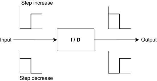
Consider a general I/D component as shown in Figure 3.8. For this element, if there is an increasing or decreasing signal, a resulting decreasing or increasing output signal will result.
Figure 3.8 Increase/Decrease component action.
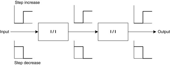
Connecting several I/I components in series, as shown in Figure 3.9, will result in an overall I/I action.
Figure 3.9 Increase/Increase components in series.
As seen in Figure 3.10, if a single I/D component is placed anywhere in the sequence the overall action is I/D.
Figure 3.10 Combined components in series.
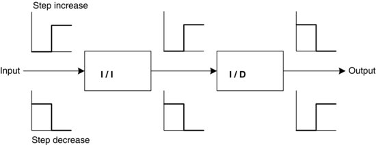
Figure 3.11 shows that when two I/D blocks are in series there is an overall I/I action. It can further be shown that whenever there is an even number of I/D blocks in a series the overall effect is I/I, and whenever there is an odd number of I/D blocks in a series, the overall action is I/D.
Figure 3.11 Increase/Decrease components in series.

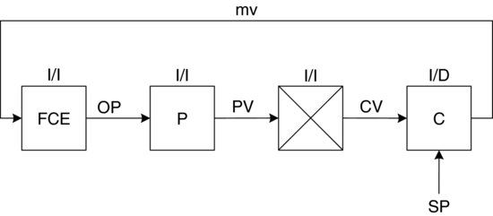
Every component in the typical loop (shown in Figure 3.12) including the sensor/transmitter, the controller, the FCE and the process is either direct or reverse acting. Recall that only negative feedback presents a viable control loop capable of maintaining stability. Thus, in the aggregate, the overall action of the control loop must be I/D or reverse acting. D/D or direct action generates, by definition, positive feedback.
Figure 3.12 Typical single input single output (SISO) loop.

Since the overall action of the control loop is determined by the action of each of the individual components, let's take a look at each of the typical control loop elements in turn.
3.4.3 Sensor/Transmitter
For the majority of applications, the sensor/transmitter produces an increasing output for an increasing input; therefore, the sensor/transmitter is typically direct acting. There are some special cases where a sensor/transmitter may be reverse acting. However, this is generally not the case, and even if it were, as will be shown later, this poses no problem.
3.4.4 Processes
Most processes are direct acting; however, they can also be reverse acting. Let us examine several major types of processes and determine the relationships between the sign of their inputs and outputs.
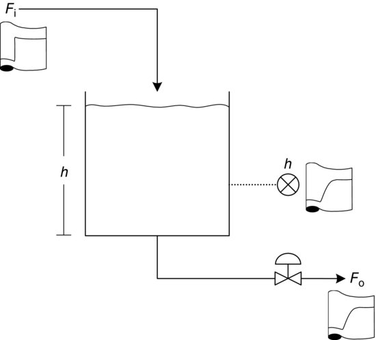
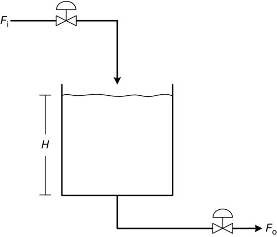
The first process is a single tank shown in Figure 3.13. For this process an increase in the input, Fi, causes an increase in the level, h, for a fixed valve position. Hence, this is a direct-acting process.
Figure 3.13 Mass flow process.
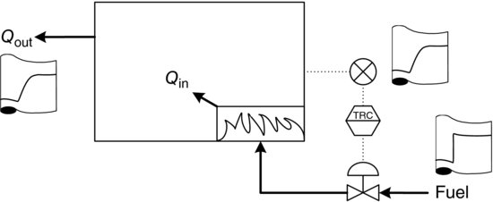
Now consider an energy flow or heating process illustrated in Figure 3.14. In this case, increasing the fuel flow results in an increase in temperature. Hence, this is also an I/I process, or direct acting.
Figure 3.14 Energy flow process.
Finally, consider the case of the reactor shown in Figure 3.15. We assume that the feed and the catalyst are mixed and the resulting chemical reaction generates heat, in other words, the reaction is exothermic. The rising temperature from this generated heat is the process output, and the cold water flow to the reactor jacket is the process input. The result is a reverse-acting process, since an increase in cold water flow will result in a decrease in reaction temperature.
Figure 3.15 Exothermic reactor.

3.4.5 Final Control Element
An FCE can be almost anything that controls the flow of mass or energy into or out of a process. It may be a motor speed control on the fan blades of an air-cooled heat exchanger, a star valve on a bin containing solids, and so on. However, in the fluid-processing industries about 90% of all FCEs are valves. Hence, it is necessary to understand the action of a control valve. For a manual control valve, as the stem position of the valve is moved upwards or open, the flow through the valve also increases, resulting in direct action. Most valve actuators in process control applications are pneumatically activated. In the case of an air-to-open actuator (fail close), an increasing air signal causes the actuator to stroke open and, therefore, the flow through the valve increases. This is direct acting. For an air-to-close actuator (fail open), an increasing air signal to the actuator closes the valve and flow decreases, resulting in a reverse-acting valve.
Therefore, in the case of the FCE being a valve, it may have either direct or reverse action depending on the actuator chosen for the valve. The desired action is chosen so that fail-safe operation is achieved. For fail-safe operation, the engineer must consider whether a ‘fail open’ valve or ‘fail closed’ valve would provide the best safety in the event of a failure. A ‘fail close’ valve simply means that if the energy supply to the valve was to fail then the valve would close, allowing no flow. Conversely, a ‘fail open’ valve opens when the energy supply fails. Cooling water to a reactor is best by an air-to-close valve. Loss of instrument air would fail the valve in the open position (because it takes air to close it), ensuring that there is sufficient cooling and preventing damage to the reactor. Conversely, the valve controlling the steam flow to a reboiler should be an air-to-open valve. Loss of instrument air here would fail the valve closed (since it takes air to open it), ensuring that the column will not overheat during the failure. See the fail-safe design section in Chapter 2 for an illustration of air-to-open and air-to-close conventions.
3.4.6 Controller
All controllers, whether implemented as stand-alone or as part of a distributed control system (DCS) application, have a switch which will allow either direct or reverse action. In general, the action of the controller is the last to be specified, since there is typically little choice in the action of the other elements in the loop. Once the other elements' actions are known, the controller action may be set such that the overall loop action is reverse acting, or I/D.
For the components shown in Figure 3.16, assume the action shown in Figure 3.17, and also assume an air-to-open actuator (I/I) for the valve.
Figure 3.16 SISO feedback control loop.
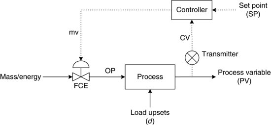
Figure 3.17 Component input/output for air-to-open actuator.
Note that the valve, process and sensor/transmitter are all direct acting. Therefore, in order to get the desired negative feedback action (I/D overall loop action) the controller must be set to reverse action.
Next consider the situation for an air-to-close (I/D) actuator, shown in Figure 3.18. In this situation, the controller must be set to direct action in order to achieve the overall negative feedback required for the loop.
Figure 3.18 Component input/output for air-to-close actuator.
3.5 Process Attributes – Capacitance and Dead Time
As we will see later in this chapter and elsewhere, the equations that govern the dynamics of some of the unit operations in typical process plants can be quite complex. Despite this complexity, many processes behave as if they were first-order systems (i.e. systems that may be described by first-order differential equations – more on that in Section 3.7), many exhibiting transport delay or dead time. Because of this, it is important to understand two fundamental process dynamic characteristics: capacitance and dead time.
3.5.1 Capacitance
Simply stated, capacitance represents a system's ability to absorb or store mass or energy. Capacitance may also be defined as the resistance of a system to the change of mass or energy stored in it, that is, inertia. A common example of a capacity-dominant process is one that stores energy (Figure 3.19).
Figure 3.19 Capacity dominated process – energy storage.

In this example the process consists of an oven which is storing heat to maintain a particular temperature, T. The gas flow creates a flow of energy in, Qin. Qout is the flow of energy to the ambient or, in other words, the heat loss to the ambient. For an increase or decrease in the valve position changing the gas flow in, the temperature would correspondingly increase or decrease. It would not, however, change instantaneously with a change in valve position. This behaviour is due to the system's capacitance.
Consider the classical capacity-dominant system shown in Figure 3.20: the surge tank. In this example the tank has a volume in which a mass of liquid is stored. Consider what would happen to the level in the tank, H, if the inflow, Fi, were increased. One would certainly expect the level to rise. However, if Fi was increased by 10%, the level would not increase to a steady-state value instantaneously. It would eventually reach a higher level, but the capacitance of the tank limits the rate of change in level, thus it takes some time to reach a new steady-state level. In other words, the tank has inertia and self-regulation. Self-regulation occurs when a process, in this case tank level, eventually lines out to a steady-state value for each input step change, rather than ramping off indefinitely.
Figure 3.20 Capacity dominated process – surge tank.
The rate of change of volume in the tank can be written as a lumped parameter model, where all the resistance to flow is assumed to be associated with the valve, and all the capacitance of the process is assumed to be associated with the tank. This model is shown in Equations 3.1 and 3.2. The basis of Equation 3.1 is the principle of conservation, mass balance in this case (i.e. what goes in must come out or get accumulated in the system):
In Equation 3.2, Q is the volumetric flow rate of water, V is the volume of the tank, A is the cross-sectional area of the tank, ρ is the density, and H is the water level. Assuming the density and cross-sectional area are constant results in Equation 3.3:
The flow, Qout, is determined by the valve characteristic V(Xp), with Xp being the valve plug-stem expressed in per cent (%) opening, the valve flow constant CV, and the square root of the pressure drop across the valve as given in Equation 3.4:
In Equation 3.4, V is a function of Xp, where V is the fraction of the total volumetric flow rate. Refer to Figure 2.21 for an illustration of how V varies with Xp for different types of valves. The symbol g is the acceleration of gravity. Substituting for Qout in Equation 3.3, which is a first-order differential equation, would result in a non-linear first-order differential which, unfortunately, has no analytical solution. The response of head (level), H, to changes in Qin or valve position could only be determined by numerical methods. However, if Qout is linearized using a Taylor series expansion about a desired operating level the first-order differential equation can be solved analytically for a disturbance in flow into the tank. This linearization for the purpose of analytical solution represents a simplification of the process dynamics. However, fortuitously most processes can be well approximated as being linear close to their operating set points. If we have designed an adequate control system, this assumption holds. Therefore we will proceed to linearize Equation 3.4 and solve it analytically. For a single variable the Taylor series can be written as shown in Equation 3.5:
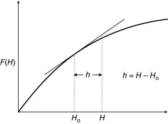
In performing a first-order linearization, shown in Figure 3.21, the higher order terms (HOT) are neglected since h = (H − Ho) is small. Setting F(H) (Equation 3.6) as a function of head, H, and substituting in Equation 3.5 results in the linear form shown in Equation 3.10:
Figure 3.21 First-order linearization.
Let
(3.7) ![]()
(3.8) ![]()
or
(3.9) ![]()
or
Let us now complete the derivation of the linear differential equation (LDE) that describes the response (also called time behaviour or personality) of the level to feed flow disturbances, starting with Equation 3.11:
At the initial or steady-state condition, Equation 3.11 can be written as Equation 3.12:
Subtracting the above two equations results in Equation 3.13:
Equation 3.13 can be rewritten in terms of deviation or variation variable, h = (Ho – H) and qin = (Qino – Qin), as shown in Equation 3.14 and in a slightly more simplified form as Equation 3.15:
In Equation 3.15, R is the resistance to flow in units of time/length2 (min/m2). Equation 3.15 can be written in the standard form for a first-order LDE (Equation 3.16):
where RA = τ = time constant (units of time).
Using the classical mathematical approach to solutions of a first-order LDE one can proceed as follows:
Equation 3.17 has a solution of the form shown in Equation 3.18 [6]:
C1 is a constant of integration evaluated from the initial conditions. Writing the LDE for the tank level in general form gives Equation 3.19:
where K = 1/A.
When there is a step input of size qin, a solution only exists for times greater than zero and is shown as Equation 3.20. C1 is evaluated at initial conditions yielding C1 = – Rqin:
The time constant, τ, characterizes the response of the first-order system and is discussed in greater detail in the next section. All higher order systems can be broken down into sets of first-order systems, and the time constants of these LDEs can be used to ascertain the relative importance of each from a dynamic response perspective. That is, the dominant, or largest, time constant will determine the speed of the response. The commonly used rule of thumb is that any subsystem with a time constant an order of magnitude (10 times) less than the dominant time constant can be described by steady-state or algebraic equations.
Some Practical Perspectives on Capacitance
While the workshop associated with this chapter will illustrate capacitance with simulation, it is worthwhile examining the practical characteristics of capacitance because, as you'll find out, capacitance can be a control engineer's best friend. A capacity-dominated system is described by Equation 3.21:
Consider a step change in qin. Mathematically, the change in h(t) begins immediately, even though the full impact of the change in qin will take some time. Now, consider a controller whose aim is to keep h(t) at some set point. Although we have not yet introduced controller algorithms and tuning, consider the most simple of control functions:
(3.22) ![]()
where mv is the manipulated variable, Kc is the controller gain, PV is the process variable, SP is the set point and e is the error. In short, corrective action carried out by the mv is simply a constant multiplier of the error.
Returning to our capacity-dominated process, the instant the PV (in this case h(t)) deviates from the set point, an error, e, will be generated, and the mv will make some adjustment. The larger the Kc, the greater the corrective action. The fact that changes in the input (mv or qin) have an immediate effect on the output (PV or h(t)) helps immensely, since the corrective action required to drive the error to zero is a straight algebraic function of the error. In the limit, as Kc approaches infinity, the error will be driven to zero and perfect control is achieved. Unfortunately, real life is not perfect, and controller gains never function at infinity. In practical terms, there is nothing that shows an absolutely ‘immediate’ response either, that is, there is no 100% pure capacitance system. However, this line of argument illustrates an important point: for capacity-dominated systems, effective control can often be achieved using simple control and large gains. As we will see in the next chapter, ‘simple control’ can be as simple as proportional-only control.
With such a simple approach to controlling capacity-dominated systems, it's easy to see why capacitance is often regarded as the control system engineer's ally. As with most things, too much is not good either. Recognize that large capacities typically increase capital cost. In addition, although capacitance acts as a buffer to upsets, if too large a volume of ‘upset material is allowed to accumulate, it can take a long time to work out of the system. Thus, the wise process designer will typically use dynamic simulations to balance the trade-offs between the capital cost optimum and the dynamic operability and control optimum.
3.5.2 Dead Time
We sometimes say that capacitance is our friend because it has the tendency to dampen out disturbances and lends itself to simple controls and straightforward tuning. Dead time, on the other hand, is typically regarded as the arch enemy of the process control engineer. Let's find out why.
Everyone has likely had the frustrating experience of showering in a very old building. The distance between the hot and cold water taps and the showerhead must be quite substantial for, when you turn the tap, it takes several seconds for you to feel the effect. Assuming you’ve been lucky enough to get the water to a comfortable temperature, there's always the inconsiderate or unaware houseguest who flushes the toilet mid shower. Quickly, you race to cut back on the scalding hot water source. There is no immediate effect and seconds seem like an eternity so you crank the valve some more. The effect of your manipulation starts to make itself known, but within a few seconds, you realize that you overdid it, and the water is suddenly freezing cold! Now your manual adjustments to the tap begin all over again, but may not settle down until a few more freeze/scald cycles play out. This example illustrates the menace of dead time. Although it may not be as entertaining, let's look at dead time mathematically and try to understand a little more about this dynamic process characteristic.
Dead time is a characteristic of a physical system that causes an input disturbance to be delayed in time, but unaffected in form. Whereas capacitance changes the form of the input disturbance (i.e. a step is filtered into a typical first-order curve), dead time is a pure delay of the input disturbance. Dead time is also referred to as transport lag, or distance–velocity lag. A typical example process is the continuous weighing system shown in Figure 3.22.
Figure 3.22 Continuous weighing system.

For instance, assume there is a conveyor belt, L metres long, moving at some velocity, v. The dead time, tDT, is calculated as shown in Equation 3.23:
If the valve is opened by some amount, increasing the material on the belt, there will be a delay equal to tDT minutes before the increased weight is sensed at the weight sensor/transmitter.
Another classic example is a liquid flowing in a pipe. If the liquid is flowing at a velocity, v, through a pipe length, l, an analogous situation exists to the weighing system. If a slug of liquid were followed through the pipe at the instant the valve is opened, it would take an amount of time tDT for the slug to go from one end of the pipe to the other. The delay times in these two cases would not necessarily be the same, but the delay effect is similar.
For a pure dead time element, assume that a step input of magnitude A occurs. The magnitude of the output step would also be A, except displaced in time by the dead time amount. The static gain, Kss, would by definition be dimensionless and equal to one, as in Equation 3.24:
Using the weighing system example of dead time, a 10 kg increase in material on the conveyor belt would result in a 10 kg increase at the weight sensor or a static gain of one. Similarly, it can also be shown that the above analysis holds for the pipe flow situation. In each of these cases a pure dead time exists since Kss = 1. However, consider the following scenario shown in Figure 3.23.
Figure 3.23 Valve/pipe flow system.

In this scenario, the input to the valve is the input to the system and the output from the system is the flow through the pipe. If the opening of the valve is increased by some per cent of valve span, A%, an increase in flow of B m3/s is delayed by an amount tDT, where tDT is the time it takes to see an increase in flow at the exit or measurement point in the pipe:
For the case shown in Equation 3.25, not only are there units but also the ratio of B to A is not necessarily one. It should be kept in mind that for pure dead time, that is, the pipe alone, Kss = 1. However, for the case where another component is involved in the dead time, the component serves to supply units to the overall gain.
Some Practical Perspectives on Dead Time
The workshop associated with this chapter will illustrate dead time with simulation and will show just how its presence makes it difficult to control a process. Let's look at why.
A system with capacitance and dead time (actually, quite a common combination) is described by Equation 3.26:
Consider a step change in qin. Mathematically, the change in h(t) will not be seen until DT time elapses. From that point on, the response in h(t) will be exactly as that illustrated in the capacity-dominated system. Consider again a controller whose aim is to keep h(t) at some set point. Also consider again the most simple of control algorithms:
(3.27) ![]()
where mv is the manipulated variable, Kc is the controller gain, PV is the process variable, SP is the set point and e is the error. Note again that the corrective action carried out by the mv is simply a constant multiplier of the error. Unlike in the capacity-dominated system, the PV (in this case h(t)) will not react immediately to the change in qin. For DT time units, h(t) will go unaffected. Only after DT time will h(t) begin to change. At that time mv will, as before, act to drive the error to zero. However, because there is no longer an instantaneous response of h(t) to the mv, the error can no longer be driven to zero by a large gain. In fact, the larger Kc becomes, the more the controller is apt to over-react. Recall our shower example! Thus, dead time, by ‘hiding’ the disturbances that lurk in the system, makes the job of rejecting disturbances extremely difficult. The larger the dead time, in proportion to the amount of capacitance, the more difficult control becomes. It is largely the presence of dead time (along with process interactions and non-linear process response) that keeps control engineers earn a decent living. In general, the more dead time can be designed or engineered out of a system the better. Also, for any given amount of dead time, the more capacitance the better. Can you think through why? Hint: 2 minutes of dead time in a chemical process with long response times (large capacitance) will not cause too much trouble. What about 2 minutes of dead time in the control loops of a jet airplane?
Let's summarize what we've just covered:
- Two types of feedback exist: positive and negative feedbacks. Only negative feedback produces stable control.
- Each element in a control loop has a particular action or sign relationship between its input and output responses. This action is important to understand, so that the action of the overall control loop produces negative feedback.
- Elements whose output increases with an increase in their input are said to be direct-acting (I/I) elements. Elements whose output decreases with an increase in their input are said to be reverse-acting (I/D) elements.
- Two important dynamic process response characteristics are capacitance and dead time.
- Capacitance acts to absorb and store mass and energy and, as such, tends to be a natural buffer to disturbances. Thus this aids in process control…to an extent. Too much can create other problems such as high capital cost and overly sluggish recovery from upsets. In general, capacity-dominated systems can be controlled with simple controls and large controller gains.
- Dead time imposes a pure delay on disturbances, effectively hiding the disturbance from the process, the measurements and the controls until it is well into the system. Dead time deteriorates controllability, especially if it is large relative to the amount of capacitance in the system with which it is associated. Dead time should generally be minimized as far as possible.
3.6 Process Dynamic Response
By this point, the reader should have an understanding of the need for and function of feedback control, understand the elements of the feedback loop and understand some of the qualitative features of the process dynamic response. While standard feedback control does not require extensive understanding of the process being controlled, some process understanding is important. In fact, the more we understand about the process, the easier our overall control system design may become. We'll touch on this more in Chapter 10 on plant-wide control. For now, let's simply take a look at the typical process dynamic responses seen in process plants. Process response determines how easily a process can be controlled and also impacts the tuning required to achieve acceptable performance.
Up to now, we have looked primarily at control as a means of maintaining the PV at a fixed set point in the presence of load disturbances. Set point changes are also types of disturbances that a control loop must be able to handle. Production rate changes, for example, require that a flow rate set point be changed. We'll use the set point change disturbance and the load disturbance as a means of illustrating process dynamic response.
As qualitatively illustrated in Figure 3.24, numerous real-time or dynamic responses are possible in returning the PV to the set point. The response labelled C1 in both cases shown above would be classed as overdamped, that is, a slow, sluggish return to set point. C2 presents the case for critical damping, that is, the fastest return to set point without oscillation. C3 is a case where there is oscillation, and C5 shows the case where instability is occurring, that is, showing a hard constraint.
Figure 3.24 Typical PV response to set point and load disturbance upsets.
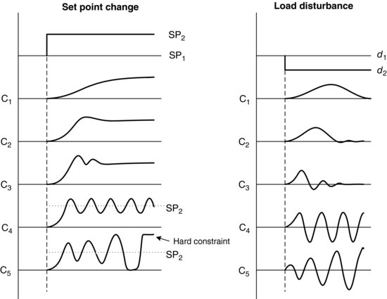
It is possible to adjust the feedback control loop to give any of the above responses. The form of the response desired depends on the process being controlled. For the most part, responses C1 to C3 would give desired behaviour since each results in a return of the process variable to the desired set point. C4 is useful in some cases for adjusting the controller, which is also referred to as tuning. Several methods developed for controller tuning depend on information gained from the uniformly oscillating loop shown in C4. C5 results in instability and is not desirable for control.
3.7 Process Modelling and Simulation
Let's examine the response of SISO control systems in further detail. In order to examine a system and its response to disturbances, an understanding of the system equations is essential and a means by which to solve these model equations. The basic steps to examining a system dynamically are to determine the equations that describe the system, solve these equations for the desired solution and then characterize the system response. The first two steps have already been done for the single tank scenario described by Figure 3.19. Now we will take this process one step further and examine the system response.
All process systems respond to various disturbances in different ways. Certain types of responses are characteristic of specific types of processes. Two of the most common personalities are those for first- and second-order systems. The single tank that was mathematically modelled in the previous section is an example of a first-order type of system.
3.7.1 First-Order Systems
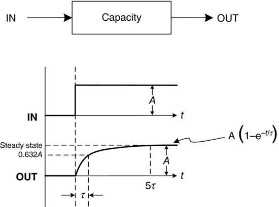
If a step input is applied to a capacity-dominated process such as a single tank, the output begins to change instantaneously but does not reach its steady-state value for a period of time. This is true of any process that is capacitive in nature. It takes approximately five time constants, 5τ, for the output of the capacity process to reach its final, steady-state value. A time constant, τ, is defined as the amount of time it takes the output of the system to reach 63.2% of its steady-state value. τ is a basic characteristic of capacity-dominated physical systems. The time constant, τ, can be defined in electrical terms as the product of the resistance times the capacitance (see Equation 3.28):
where R is the resistance in the system and C is its capacitance with the units of each being appropriate for the system in question to make the time constant units be units of time, that is, seconds, minutes and so on.
Figure 3.24 demonstrates the step response behaviour of the single tank example discussed previously. The equations describing the tank system were developed in the previous section and are clearly first-order differential equations. Any single-capacity system is typically a first-order system and will respond in the same manner illustrated in Figure 3.25.
Figure 3.25 First order system response to a step input.
3.7.2 Second-Order and Higher Order Systems
Higher order responses are the result of multi-capacitance processes that contain vessels in series, fluid or mechanical components of a process that are subjected to accelerations causing inertial effects to become important or the addition of controllers to a system. In a chemical plant, higher order systems that result from a combination of capacities and controllers are very common. Typical examples are reactors in series, heat exchangers and distillation columns. In the case of distillation columns, when controllers are attached to the column, very high order, non-linear differential equations result when the system is mathematically modelled. Mechanical component time constant and natural frequencies are very small relative to the process time constants and frequencies and, as such, the resultant effects are typically minor.
In order to get a feel for what a second-order system looks like, we will first examine a familiar component from the SISO system. An integrated part of the SISO system that results in a second-order differential equation is the diaphragm-operated control valve shown in Figure 3.26.
Figure 3.26 Diaphragm operated control valve.
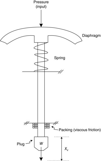
In order to derive the system equation we first apply Newton's second law, which states
(3.29) ![]()
The spring force, viscous friction and acceleration terms are described as follows:
(3.30) ![]()
(3.31) ![]()
(3.32) ![]()
The force is a function of time equal to the pressure applied to the top of the valve, P(t), times the area, A. This term is referred to as the forcing function:
where Xv is the position of the plug (output), P is the pressure at the input, K is the spring constant, b is the coefficient of viscous friction and W is the weight of the plug and stem.
Equation 3.33 is obviously of the second-order differential form and, hence, when simulated will give a typical second-order response. To better understand what type of response these second-order systems will display we will examine another common system and generalize its equations. The closed form solution is best illustrated by an example that is familiar, namely the spring, mass and damper system presented in Figure 3.27. Note that this is really just a simplification of the control valve example just cited.
Figure 3.27 Spring, mass and dash pot (damper) system.

If we perform the same analysis on this system as on the previous one, the following equation is obtained describing the system where both the force and displacement are positive in the upward direction:
Since the rest, or equilibrium, position YR is constant, Equation 3.34 can be rewritten in terms of the displacement from the rest position, y. In this manner, we will be looking at variations about the equilibrium position, that is, steady state. This is a common approach in system analysis because analysis of even non-linear systems about a steady state results in a linear system, that is, ordinary differential equations (ODEs):
Substituting Equations 3.35, 3.36 and 3.37 into Equation 3.34 results in the following:
Another point to be made about the analysis of our system is that we used the lumped parameter simplification. All the mass, friction (dash pot) and self-regulation (spring) are considered to be lumped at one point. The use of a lumped parameter model instead of a distributed parameter simplifies the mathematics of the model by producing ODE instead of partial differential equations.
In order to solve the second-order equation which will give the position of the mass as a function of time we need the specific set of initial conditions. For a second-order differential equation we use the following conditions:
(3.39) ![]()
(3.40) ![]()
In the simplest case the forcing function, f(t), can be set to zero. The resulting homogeneous differential equation can be found by finding the roots of the characteristic equation, given in Equation 3.41:
For a second-order algebraic, these roots are given by Equation 3.42 and are called the eigenvalues:
Provided that the roots are all real and unique, the solution is as follows:
(3.43) ![]()
C1 and C2 are constants evaluated using the two initial conditions. The resulting plot of y versus t will have one of the general responses shown in Figure 3.27. The system descriptive parameters, in this case C, K and M, govern the particular response or behaviour of the system.
Second-order systems are very common in the chemical industry and have recently received much attention. The equation describing a second-order system such as the spring, mass and damper example can be further generalized by dividing Equation 3.38 by M:
Equation 3.44 can be further generalized by defining the following terms:
(3.45) ![]()
(3.46) ![]()
These generalized terms then characterize the response of the system. The first term, ωn, is called the undamped natural frequency, while ξ is known as the damping coefficient. Note that the natural frequency of the system is proportional to K (the tendency to self-regulate) and inversely proportional to M (the capacitance or inertia of the system). Note also that damping is directly proportional to C (system friction), but inversely proportional to M (capacitance or inertia) and K (self-regulation). Understanding how the frequency and damping in a system are affected by these fundamental process characteristics can be useful as the control scheme for a real chemical process is undertaken. Remember that sometimes some simple changes in the process itself can make the job of designing and tuning a regulatory control system much simpler!
The solution to Equation 3.44 can again be found by finding the roots of the characteristic equation, shown in Equation 3.47:
(3.48) ![]()
(3.49) ![]()
(3.50) ![]()
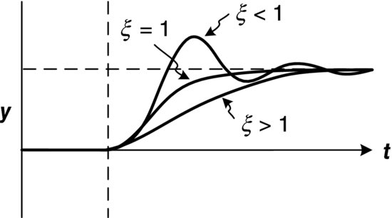
The response of the system will depend mainly on the damping coefficient, ξ. When ξ < 1, the system is underdamped and has an oscillatory response. The smaller the value of ξ, the greater the overshoot. If ξ = 1, the system is termed critically damped and has no oscillation. A critically damped system provides the fastest approach to the final value without the overshoot of an underdamped system. Finally, if ξ > 1, the system is overdamped. An overdamped system is similar to a critically damped system in that the response never overshoots the final value. However, the approach for an overdamped system is much slower and varies depending upon the value of ξ. These typical responses are illustrated in Figure 3.28.
Figure 3.28 Typical second order response.
Now let us examine the case of multiple capacities in series. Consider two non-interacting tanks in series, shown in Figure 3.29.
Figure 3.29 Two non-interacting tanks in series.

The mass balances for tank 1 and tank 2 are given by Equations 3.51 and 3.52, respectively:
If linear resistance to flow is assumed for the valves in the system the following equations are obtained:
Now substitute Equations 3.53 and 3.54 into Equations 3.51 and 3.52 to give
(3.55) ![]()
Differentiating Equation 3.56 with respect to time and re-writing h1 in terms of h2 gives a second-order ODE:
We can then apply the same generalization to Equation 3.57 as we did for Equation 3.44. This generalization gives the following:
(3.58) ![]()
(3.59) ![]()
Now that the equations describing the system have been developed, the system can be simulated and its response to disturbances examined. Based on the equations developed for the single tank and the non-interacting tanks in a series, what type of response would the level in the first and second tanks display?
3.7.3 Simple System Analysis
Often questions arise in the design of a process concerning the controllability of the system, alternative control schemes and variations in the process design to achieve quality and/or throughput. In order to answer such questions, without building the plant, it is necessary to have available a rigorous mathematical model or modelling system. Once the system, which includes plant unit operations and controllers, is modelled and simulated, the effect of various parameters and control schemes can be predicted and evaluated.
The determination of the process mathematical model is often the most difficult and time-consuming step in control system analysis. This is a result of the dynamic nature of the process, in other words, how the system reacts during upsets or disturbances. The problem is further complicated by process non-linearities and time-varying parameters. To illustrate the modelling procedure we will look at developing a model for a shell and tube heat exchanger with temperature control [7], shown in Figure 3.30.
Figure 3.30 Typical process schematic of shell and tube heat exchanger.

Constructing a Word Block Diagram
Before starting to analyse the process, it is helpful to construct a system block diagram (Figure 3.31). The purpose of the block diagram is to identify the components of the SISO and all load disturbances. Recall that a simple SISO feedback loop is comprised of four basic units:
Figure 3.31 Word block diagram of shell and tube heat exchanger.

In order to limit the complexity of the analysis all parameters will be assumed to be constant. The procedure will be to develop the ODEs for each of the components and combine these into a system model.
Valve Top and Positioner
One approach to modelling SISO loop components is through step testing. For the valve and valve positioner a first-order ODE such as the following may be determined:
where X is the valve stem position, P1 is the valve top pressure (that opens and closes the pneumatic valve, after the controller compares the set point to P3), τ is the first-order time constant, K is the steady-state gain and t is the time. For this valve and valve position, the steady-state gain is K = 0.179 mm/kPa and the time constant is τ = 0.033 minute. Therefore, we can write Equation 3.60 as follows:
Equations 3.60 and 3.61 are written in terms of variation variables. Variation variables represent a change from or about a steady-state level of the variable. The gain was determined by dividing the valve stem travel by the pneumatic signal range, which is 14.3 mm divided by 80 kPa (the range in this case is from 20 to 100 kPa). The time constant of 0.033 is determined experimentally using a step input signal (discussed previously under Section 3.7.1).
Sensing Element and Transmitter
These components can also be represented by a first-order ODE, as in Equation 3.62. In most cases this is an adequate representation for SISO loop analysis:
where P3 is the pressure signal from the temperature sensor/transmitter to the controller and θ2 is the exit water temperature. The steady-state gain, K, is determined from the sensor/transmitter ranges, which are 0–100°C input and 20–100 kPa output. This results in a gain of 0.80 kPa/°C.
The time constant of the measuring element equals the thermal resistance times the capacitance. The thermal resistance can be modelled as a function of area and the heat transfer film coefficient:
where Rt is the thermal resistance (°C/kW), A is the surface area (m2) and h is the film coefficient (kW/°C m2).
The thermal capacitance is a function of mass and specific heat:
where Ct is the thermal capacitance (kJ/°C), W is the mass of sensing element (kg) and C is the specific heat (kJ/kg °C).
The time constant, which has the units of hours as a result of the units of the film coefficient, can then be found using Equations 3.63 and 3.64:
(3.65) ![]()
Once the sensing element has been selected, its area, weight and specific heat are fixed. Therefore, τ is only a function of h. If the manufacturer provides a time constant, τ, for a given set of conditions, other τ can be estimated based on the new conditions. If the system properties are about the same as those the manufacturer used during the step tests, h will primarily be a function of fluid velocity. Assuming that the bulb has a time constant over a limited velocity range as follows:
(3.66) ![]()
where τ is the time constant (seconds) and v is the fluid velocity (m/s).
Thus, for a fluid velocity of 0.686 m/s, the time constant of the sensing element is 0.024 minute (1.43 seconds).
Process Model
The process model can be determined either from first principles (the mechanistic approach) or by ‘black boxing’. Mechanistic approaches attempt to model transient energy and mass balance. Black box models are often even simpler and describe the input–output behaviour with no recourse to conservation principles. Using a lumped, linear system analysis approach, we assume that a local linear model about the operating set point holds and the heat exchanger is modelled as one lump (lumped parameter approach) in which a small change in the valve stem position, ΔX, and its effect on the outlet water temperature, θ2, are predicted. A change in X results in more or less steam entering the shell, which changes the energy input to the heat exchanger. This change in energy input is accounted for by a change within the exchanger and a change in the energy leaving the exchanger. If the inlet water flow rate, Qw, and inlet temperature, θ1, are constant, any change in energy will show up as a change in water outlet temperature, θ2.
The steam flow, Qs, through the valve can be modelled as follows:
(3.67) ![]()
where Qs is the steam flow (kg/s), X is the valve stem position or travel (mm) and Ps is the steam pressure (kPa).
In terms of variation variables, the change in steam flow can be modelled as follows:
(3.68) ![]()
where
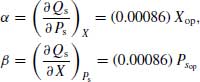
and op is the operating point around which X and Ps are defined.
If one assumes saturated steam in the shell, there is a unique relationship between changes in steam pressure, Ps, and changes in steam temperature, θs:
(3.69) ![]()
The coefficient γ can be evaluated from steam tables at the shell nominal operating pressure of 432 kPa; refer Table 3.1. As can be seen from Figure 3.32, at an operating pressure of 432 kPa, γ can be linearized to give a value of 11.0 kPa/°C.
Table 3.1 Saturated steam temperature.
| Ps (kPa) | θs (°C) |
| 300 | 133.5 |
| 350 | 138.9 |
| 400 | 143.6 |
| 450 | 147.9 |
| 500 | 151.8 |
Figure 3.32 Steam pressure versus steam temperature.

An energy balance on the shell using the principle of energy conservation can be written as follows:
(3.70) ![]()
where m is the latent heat of condensing steam (kJ/kg; 2129 kJ/kg for this example), Wt is the tube weight (kg), Ct is the specific heat of the tube material (kJ/kg °C; 0.5 kJ/kg °C for this example), Ws is the shell weight (kg; 19.6 kg for this example), Cs is the specific heat of the shell material (kJ/kg °C), ht is the tube side film coefficient (kW/°C m2), At is the tube area (m2; htAt = 0.376 kJ/s °C), θs is the steam temperature (°C) and θ2 is the outlet temperature (°C).
The shell-side energy balance contains a number of simplifying assumptions. The shell-side heat transfer film coefficient is assumed to be negligible, thus the temperatures of the tube and shell walls are equal to the condensing steam temperature. Shell steam capacity is also assumed negligible due to the small volume. Losses to the atmosphere are neglected, that is, the shell is well insulated.
In the development of a mathematical model the validity of assumptions is always debatable and depends on the use of the model, required accuracy, equipment size and configuration. These need to be considered in light of where and how the model is to be used.
The water temperature was taken as the average between the inlet and outlet temperatures. This assumption is valid since the inlet temperature is assumed to be constant; hence the change in the average water temperature is half the change in the outlet water temperature. An energy balance for the water flowing in the tube side results in the following equation:
(3.71) ![]()
where Qw is the water flow into the tube (kg/s), Cw is the specific heat of water (kJ/kg °C; 4.2 kJ/kg °C for this example), Ww is the water weight in the tube (kg), ht is the tube-side film coefficient (kW/°C m2), At is the tube area (m2), θs is the steam temperature (°C) and θ2 is the outlet temperature (°C).
Controller
If we use a standard PI controller, it can be modelled using Equation 3.72. A PI controller takes remedial action proportional to the magnitude of both the error and the integral of the error and is rigorously defined in Chapter 4:

where Kc is the controller gain, an adjustable tuning parameter of the controller; Ti is the integral time, another adjustable tuning parameter of the controller; and Δe is the error and defined as the difference between the measured variable and the set point, which is 65°C for this example:
(3.73) ![]()
Response
The time response of the outlet temperature to various load disturbances can be determined by integrating the set of ODEs, as developed previously. This can be accomplished by using one of the standard mathematical software packages, such as MATLAB™ [8]. For clarity these equations are repeated below with their original numbering and are in the order that they appear in the control loop, with the values of the constant parameters shown:
(3.61) ![]()
(3.68) ![]()
(3.69) ![]()
(3.70) ![]()
(3.71) ![]()
(3.62) ![]()
(3.72 and 3.73) 
The resulting response for this system to a PI controller set point change is shown in Figure 3.33.
Figure 3.33 Typical response for a PI controller set point change.
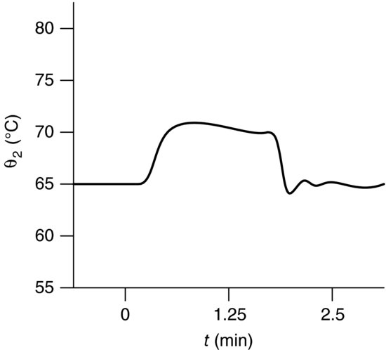
The response in Figure 3.33 is based on a simple linear lumped parameter model; thus for large disturbances or set point changes that exceed the limits of the linear assumptions and other operating point, quite different responses will be obtained.
3.7.4 Classical Modelling for Control Approaches
The previous simple analysis example follows a pre-computing classical approach where a simple linearized lumped parameter model of the system was developed. In the pre-computing or classical approach this simple model was solved by the application of analytical methods such as Laplace transforms and frequency response analysis. For completeness these methods will be briefly introduced here. The interested reader should refer to the texts that take this pre-computing classical approach such as Coughanowr and Koppel [9], Luyben [10], Harriott [11], Murrill [12] and Shinskey [5].
Laplace Transforms
Solving Laplace transforms is a process of leaving the time domain where a differential equation may be too difficult to solve without a computer and entering the Laplace domain where the transform of that differential equation is readily solved and then coming back into the time domain with the inverse transform of the Laplace domain solution.
Differential equations may be classified as per the taxonomy in Figure 3.34.
Figure 3.34 Differential Equations.
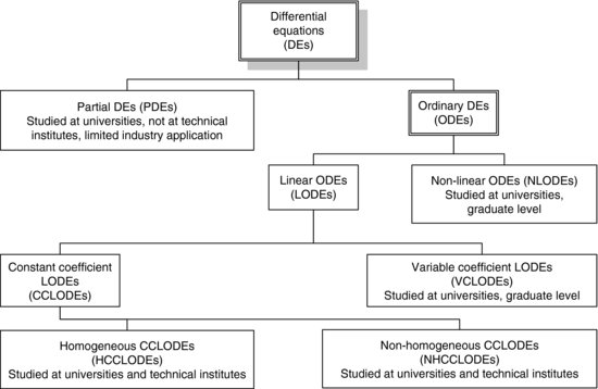
HCCLODEs and NHCCLODEs are of the form given in Equation 3.74:
Mathematically equations of this type comprise a very narrow class of equations, but they represent quite a number of simple physical systems. For homogeneous systems, f(t) = 0. The simplest HCCLODE is given by Equation 3.75:
An example of a physical system represented by Equation 3.75 is the linearized equation for change of level h in a cylindrical tank of cross-sectional area A, with no input flow, and output flow regulated by a valve of resistance R:
(3.76) ![]()
Other examples are the voltage (V) in a resistor capacitor (RC) circuit without an applied input voltage, and the change of current (i) in a resistor inductor (RL) circuit without an applied input current, as described by Equations 3.77 and 3.78, respectively:.
In the above examples, the equations describe physical systems with one energy storage or capacitance element and one energy-dissipating or resistive element and are not subject to external forces.
Solving a first-order equation such as the above example can be done using analytical integration.![]() , from which
, from which![]() , where y(0) is the initial energy. However, this is the only type of equation that can be solved thus.
, where y(0) is the initial energy. However, this is the only type of equation that can be solved thus.
To solve this equation using Laplace transforms we use the following definition of the Laplace transform (Equation 3.79) and standard transforms of functions, for example, Coughanowr and Koppel [9]:

We operate like so: ![]()
or![]() , from which
, from which ![]() and
and![]() .
.
Note that coming out of the Laplace domain is more difficult than entering it and extensive use of partial fractions is necessary for this job.
Transfer Functions
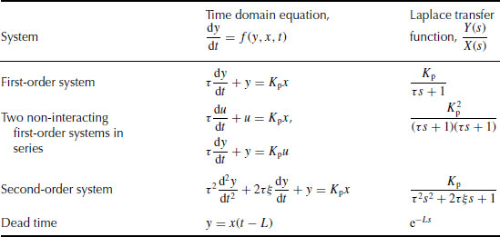
A transfer function is the relationship between the input and the output of a system. In classical control systems literature that makes use of Laplace transforms, extensive use is made of Laplace transfer functions. Table 3.2 presents the transfer functions of common process systems dynamics.
Table 3.2 Transfer functions of common process systems dynamics.
Frequency Response
Frequency response analysis is another classical tool that has been used in the analysis and design of process control systems. The Laplace variable s is replaced by jω, where ![]() and ω is the radian frequency. The frequency response is then plotted using an Argand diagram approach.
and ω is the radian frequency. The frequency response is then plotted using an Argand diagram approach.
For example, consider the frequency response of the first-order process given by the transfer function, ![]() .
.
The Laplace variable s is replaced by jω and converted to polar form. Then the amplitude ratio (AR) and phase (α) are computed via Equations 3.80 and 3.81:
These can be plotted either on Bode graph paper or Black–Nichols graph paper, and if converted to decibels (db) via ![]() , the response can be plotted on semi-log and polar graph paper.
, the response can be plotted on semi-log and polar graph paper.
The concepts of gain margin and phase margin are used for control system design using frequency response analysis. Gain margin is the additional amount of gain that would destabilize the system. Phase margin represents the additional amount of phase lag required to destabilize the system. Both gain margin and phase margin can be obtained from the open loop Bode diagram of the system. Typical design specifications are that the gain margin should be greater than 1.7 and the phase margin must be greater than 30°.
3.7.5 The Modern Modelling for Control Approach
The modern approach to process modelling for process control that this book takes and as described in Chapter 1 is to make use of simulation tools and computer-based design packages that avoid the limitations imposed by the analytical design methods, namely abstraction, linearization and simplification, for example, Allen [13].
Mathematical models imbedded in today's simulation software provide a means to handle both variations in operating level and process non-linearities. The important result is not the controller settings but the ability of the designer to manipulate process parameters to meet process specifications at a minimum cost. This can only be achieved by developing a deep understanding of the process and the system, which includes the process and the controllers.
References
1. Bequette, B.W. (1998) Process Dynamics: Modeling, Analysis, and Simulation, Prentice Hall, New Jersey.
2. Riggs, J.B. (1994) An Introduction to Numerical Methods for Chemical Engineers, 2nd edn, Texas Technical University Press, Texas.
3. Smith, C.A. and Corripio, A.B. (1997) Principles and Practice of Automatic Process Control, 2nd edn, John Wiley & Sons, New York.
4. Downs, J.J. and Doss, J.E. (1991) Present status and future needs – a view from North American industry. Proceedings of 4th International Conference on Chemical Process Control, Padre Island, Texas, 17–22 February, pp. 53–77.
5. Shinskey, F.G. (1996) Process Control Systems: Application, Design and Tuning, 4th edn, McGraw-Hill, New York, NY, p. 4.
6. Johnson, R.E. and Kiokemeister, F.L. (1978) Calculus with Analytical Geometry, 6th edn, Allyon and Bacon, Boston, p. 737.
7. Wilson, H.S. and Zoss, L.M. (1962) A practical problem in process analysis. Control Theory Notebook, ISA Journal Reprints, pp. 25–28.
8. MATLAB™ (1999) Version 5.3, The MathWorks Inc., Natick, MA, USA.
9. Coughanowr, D.R. and Koppel, L.B. (1965) Process System Analysis and Control, McGraw-Hill.
10. Luyben, W.L. (1973) Process Modeling, Simulation, and Control for Chemical Engineers, McGraw-Hill, New York.
11. Harriott, P. (1964) Process Control, McGraw-Hill, New York.
12. Murrill, P.W. (1967) Automatic Control of Processes, International Textbook.
13. Allen, R.M. (2002)Variability and the infinite process control horizon. Proceedings of 9th Asian Pacific Confederation of Chemical Engineering Congress and the Australasian Chemical Engineering Conference 2002, Christchurch, New Zealand, 29 September–3 October, pp. 113–114.