
Workshop 4
Feedback Control
Nothing comes from doing nothing.
—Shakespeare
Introduction
Prior to attempting this workshop, you should review Chapters 3 and 4 in the book.
The previous workshop introduced the concepts of capacitance and attenuation. These are ‘natural’ characteristics of a system, as are dead time and the process time constant. Now that we have a basic understanding of the way processes behave, we can apply this knowledge to control the process response.
Once the process personality is understood, we can manipulate process flows to maintain a desired variable at constant conditions, which are called set points. This is known as feedback control, where the value of a variable is ‘fed back’ to a controller which manipulates another variable according to the difference between the controlled variable and its set point.
Key Learning Objectives
- Attenuation decreases as the gain increases.
- Adding integral action to an integrating process (level control) can become a disturbance generator rather than a disturbance smoother if not properly tuned.
- Level loop tuning is always dependent on the system characteristics.
- If the hold-up is too small to get good flow smoothing, reduce Kc and add integral action to ensure that the level stays in the tank (Kc×Ti = 4.0).
- If the hold-up time is long, you do not need any integral action.
- If the level is cycling, increase Kc and decrease Ti (this is the opposite of other loops).
Tasks
1. Low-Capacity, No Dead Time Process
In the previous workshop, you should have built the system shown in Figure 4.1. Check that you still have the Wilson property package specified. The only components required are water and methanol, and O2 and N2 for the vapour phase hydraulics. The inlet temperature should be 30°C, while the heater outlet should be fixed at 70°C. Initially, we wish to analyse a process without dead time so you will need to delete the pipe segment that you added in the previous workshop. Retain the strip charts that you set up previously. If they have been deleted, rebuild them to contain the following variables: feed temperature, separator outlet temperature, heater duty, feed molar flow. Select suitable ranges for each variable.
Figure 4.1 Low-capacity, no dead time process.
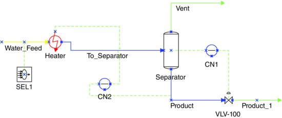
The results from the previous workshop indicated that processes with low capacitance and relatively long disturbance period have the lowest attenuation and are in most need of process control. Hence, for this portion of the workshop you will need to use a low-capacity process, so adjust the separator level accordingly. Your simulation should still contain a transfer block operation, which adds noise to the system. Set the feed water temperature disturbance period to 30 minutes and its amplitude to 25°C.
Now add a controller for the separator outlet temperature. The controller should directly manipulate the heater duty between 0 and 1×10⁶ kJ/h. Please note that since VMGSim does not support direct control on energy streams, you will need to select the manipulated variable from the heater InQ. The PV range should be 0–100°C, and the set point should be 70°C to match the steady-state conditions. Set the controller gain, Kc, to 1.0, but leave the integral time and derivative time blank. Make sure that you correctly specify whether your controllers are direct acting or reverse acting so that the controller will open/close the valve when required and not vice versa. Finally, set the controller to automatic.
The previous workshop demonstrated that capacity-dominated processes have significant disturbance rejection (attenuation) properties without requiring any form of process control. This is called open loop attenuation. Controllers can usually increase the attenuation of process systems. When operated in ‘automatic’, the additional attenuation is called closed loop attenuation. When in ‘manual’ the system behaves as it would without the controller present.
- Vary the gain to achieve the maximum closed loop disturbance attenuation. How effective is the controller in rejecting disturbances not already rejected by the natural attenuation of the process?
- What happens when the controller gain gets very high? Is there a limit to how much you can increase the gain?
2. Process with Dead Time
Capacity-dominated processes are relatively easy to control. However, the presence of dead time makes the control problem more difficult. We can demonstrate this by adding a pipe segment to the system shown in Figure 4.1 in order to simulate dead time. The pipe segment should have a length of 2.0 m, a total volume of 0.5 m3 (dead time = 10 minutes) and a pressure drop of 0 kPa. The process layout is presented in Figure 4.2. Remember that you want to work with a capacity-dominated process, so ensure that the separator level is set accordingly. Also remember to save your case after setting up the controller, since an unstable system may stop the integrator and the system will be difficult to restart.
- What is the maximum attenuation for the process with dead time?
- Is there an optimum/maximum gain that maximizes process attenuation?
- Fix the controller gain at Kc ≈ 10 and calculate attenuation for dead times of 2, 5, 10 and 20 minutes. Vary the size of the PFR to change the amount of dead time in the system. Record the results in Table 4.1.
Table 4.1 Process attenuation with dead time.
| Dead time (minutes) | ΔT – product temperature (°C) | Attenuation |
| 2 | ||
| 5 | ||
| 10 | ||
| 20 |
Figure 4.2 High-capacity process dead time.

3. Proportional-Only Control
We have found that feedback control can provide good attenuation of process disturbances provided that the dead time is not too great. The ability to provide attenuation to a process is sometimes called disturbance rejection. However, disturbance rejection is only one of the requirements of an effective controller. The other main requirement is that we should be able to change the set point whenever we want and have the controller manipulate the process so that the controlled variable continues to match the set point. This is sometimes referred to as controller performance. These two parameters, disturbance rejection and controller performance, are used to assess the effectiveness of a controller.
Eliminate dead time from the system by deleting the pipe segment or setting its volume to a very low value and pause the feed temperature disturbance to remove the noise from the process. Starting with a gain of 1.0, interactively change the separator outlet temperature set point to 80°C.
- Where does the separator outlet temperature stabilize? The difference between this value and the set point is called offset.
- Plot the relationship between offset and the controller gain.
- Can you explain the relationship shown on the plot between offset and the controller gain in terms of proportional-only controller equation given in Equation 4.1?
4. PI and PID Control
The feedback controller we have employed to this point has only contained one term: gain. As suggested above, this type of controller is called proportional-only controller, which suffers from the problem of offset. Offset can be reduced with high values of gain, but sometimes this makes the controller unstable, particularly when there is dead time in the system. We can eliminate offset by introducing another term to the controller equation: integral time. The control equation for a proportional-integral (PI) controller is
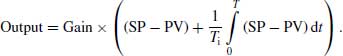
- How does PI control eliminate offset? Use Equation 4.2 to help explain.
Add integral time to your controller, starting with Ti = 1.0 minutes, and check that it eliminates offset for set point changes, both with and without dead time in the system. Interactively change the feed rate to determine how effective the controller is at disturbance rejection, that is, step response testing.
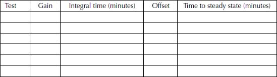
- Summarize your results for PI control in Table 4.2. Record under the ‘Test’ column the details of each type of step test performed, that is, 30–40 kmol/h.
Table 4.2 PI controller optimization.
Integral action can be slow since it relies on the integral of the error being large, where the error is the difference between the set point and the process variable. Proportional action usually provides the ‘muscle’ for the controller. However, too much proportional action creates instability. In some circumstances, PI controllers are not sufficiently fast, making third controller action necessary. This term is called derivative time and can sometimes be introduced to speed up the response time of the controller. The control equation for a proportional integral derivative (PID) controller is
(4.3) 
Derivative time increases the controller response when the controlled variable is moving away from its set point most quickly, that is, straight after a disturbance has affected the system. Apart from increasing the responsiveness of the controller, derivative action also reduces oscillation. Derivative action can be very effective under some circumstances but very damaging under others. For example, if the system is essentially stable but there is a small amount of process noise (usually very high frequency), the derivative action will interpret the noise as being the start of a large disturbance and will make large changes in the manipulated variable which are clearly not required.
Add derivative action, starting with Td = 1.0 minutes, to your system to determine whether or not it improves the controller effectiveness for this example.
- Optimize controller performance by varying the three controller parameters. Consider the responsiveness to the process disturbances and the ability to track a set point. Record your results in Table 4.3. Under ‘Test’ column, record the type of step change test performed.
Table 4.3 PI controller optimization.

5. Averaging Level Control
Surge drums and intermediate product tanks are critical parts of any process system. Their principal purpose is to provide hold-up and capacitance to smooth out flow disturbances so they do not carry through to downstream process units. This function must be recognized and it is frequently overlooked in many operating plants. A consequence of this function is that the level in the surge drums and intermediate tanks should NOT be tightly controlled. Tight level control will transmit flow disturbances to downstream units and negate the effectiveness of the surge volume. The level controller must only control the level between the low limit (when the tank/drum approaches empty and thereby risks damaging the outlet pump) and the high limit (when the tank overflows). Intentional loose level control is called averaging level control.
One exception to the rule of averaging level control for surge drums is in the case of distillation column hold-ups. Averaging level control should not be used to control the reflux drum level or the reboiler sump level. Tight level control is required for these vessels to maintain the integrity of the column material balance so that changes in the reflux and reboiler duty will have the desired effect on product compositions and yields without introducing additional lag to the system.
In order to better understand how averaging level control works, build a simple system consisting only of a 2 m3 separator. The feed to the separator should be 250 kmol/h of water at 25°C and 100 kPa. Add a level controller and enter a set point of 50%. Finally add a feed disturbance using a selector block unit operation set up to vary the feed rate sinusoidally with an amplitude of 25 kmol/h. You need to be aware of the control valve CV value.
- Test the following combinations of PI control for the separator level controller for the range of disturbance periods given in Table 4.4:
- Which combination of gain and level control provides the best disturbance attenuation?
- Are there any problems with using a very low gain?
- Are there any problems with using a proportional-only level controller?
Table 4.4 Averaging level control.

Present your findings on CD, DVD or thumb drive in a short report using MS-Word. Also include on the submitted media a copy of the VMGSim files which you used to generate your findings.