Workshop 3

Process Capacity and Dead Time

Knowledge is a treasure but practice is the key to it.

—Thomas Fuller

Introduction

Prior to attempting this workshop, you should review Chapter 3 in the book.

This workshop will illustrate the effect on the process response of the three key process dynamic parameters: process gain, process time constant and process dead time. You will also explore the impact that capacitance or ‘lag’ has on these process parameters.

Key Learning Objectives

Tasks

1. System Identification

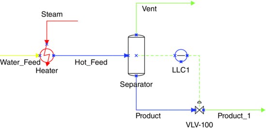
The process used for this workshop is shown in Figure 3.1. Build a simulation of this system with the following basis:

Figure 3.1 Illustrative capacity-dominated process.

Property Package: Wilson.

Components: water, methanol, N2 and O2 (N2 and O2 are used to simulate the air in the separator that displaces liquid when the separator level drops).

Switch to the simulation environment and add a feed stream with the following data: Flow = 100 kmol/h, Temperature = 30°C and Pressure = 200 kPa, Composition: water = 50%, methanol = 50%, O2 = 0% and N2 = 0%.

Add a heater and a separator to your flow sheet and specify the volumes of 0.1 m3 for the heater and 2 m3 for the separator. The duty stream ‘Steam’ should heat the stream to about 70°C. The hot mixture is then stored in the separator for future use.

‘System identification’ is the term used to define a procedure to characterize the process response. In this case, system identification can be accomplished by adding a level controller to the separator (add a controller and flow control valve on the liquid outlet stream), with a set point of 50%, adjusting the steam flow to the heater in steps, up and down, and then observing the temperature response on the strip chart. This is termed ‘step response testing’.

Figure 3.2 illustrates a typical step-test response for a first-order system. The relevant process parameters of gain, Kp, time constant, τ, and dead time, tDT, for this first-order process are shown and can be calculated as follows:

(3.1)

where Output is the separator temperature change/temperature transmitter span and Input is the steam rate change/steam valve span.

• In order to check how linear the process is it is necessary to determine if the gain is the same regardless of the steam rate and to see if the magnitude of the gain is unchanged for increases and decreases in steam duty. Do this by using the step-testing method described above and Equation 3.1.

Figure 3.2 System step response.

2. Capacitance

Now we will examine how the gain, time constant and dead time vary for different separator levels or different amounts of capacitance in the process shown in Figure 3.1.

• Make step changes in the steam rate for three different separator level set points of 5%, 50% and 95%. Calculate the gain, time constant and dead time for the three different process capacities. Present your results in Table 3.1 and then plot a graph of each of the time constant and gain versus separator level.

Table 3.1 Summary of process parameters.

3. Attenuation

As has been indicated in the book, an object of both the process and the control system is to reject or at least minimize the effect of disturbances. In order to quantify disturbance rejection the term ‘Attenuation’ has been borrowed from the electrical/mechanical engineers and is defined as follows:

(3.2)

For example, if the separator temperature varies with an amplitude of 5°C and the input temperature disturbance has an amplitude of 25°C, the attenuation is (1 – (5/25)) = 0.8 or 80%.

In VMGSim, to generate a sinusoidal feed temperature a selector block unit operation is used. From the PFD tab, drag the selector block onto the flow sheet. Choose the ‘Hand Sel’ option under ‘Selector Mode’, select ‘Sine wave’ under ‘Output Bias Fn’ and specify the magnitude as well as the period. Connect to the inlet feed at ‘output’ region and select appropriate unit for the signal as required. Then, you need to enter the value for ‘x’ as 30, the input scale ‘m’ value for 1 and leave the input bias ‘b’ value for 0. The selector block automatically calculates the scaled input ‘y’ and the scaled output ‘z’. Finally, start the integrator to see whether the selector block can properly generate the sine wave for the inlet temperature as expected. If your output value is still wrong or biased, make sure the ‘Output Scale’ is specified as 1, and ‘Output Bias’, ‘Noise Magnitude’ and ‘Noise Decay Time’ are specified as 0.

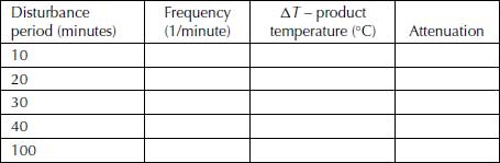
• Complete Tables 3.2–3.4 for each separator level and then plot the Attenuation in percent versus Disturbance Period in minutes, with a curve for each level.

Table 3.2 Attenuation for level at 5%.

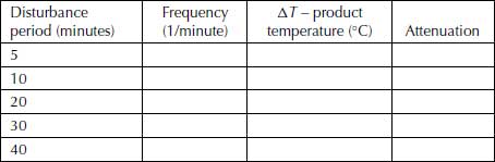
Table 3.3 Attenuation for level at 50%.

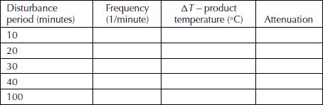
Table 3.4 Attenuation for level at 95%.

[Note: You will need your results from this section of the workshop for later workshops so remember to save a copy of the results for yourself.]

4. Dead Time

In this section of the workshop the dynamic characteristics of processes with capacitance and appreciable dead time will be studied. The process you will work with is the simple feed heater and a separator acting as a storage tank, shown in Figure 3.1, except that additional equipment will be added between the heater and the separator. The additional equipment will be a pipe segment with a volume of 0.3 m3 and length of 2 m, which gives a dead time of 6 minutes for the specified inlet flow rate. Figure 3.3 shows an example of what this process should look like. The objective is to see how dead time affects the temperature response of the warm solution leaving the separator.

Figure 3.3 A process containing dead time.

Again this simple example is illustrative of many real plant situations. Even the time it takes for the fluid to move through pipes between connecting items of equipment is an example of dead time. A sensor located at a distance from a vessel such as a reactor introduces process dead time. The time it takes for a process analyser to sample a process stream and measure a particular property and the time it takes for a manual sample to be taken to the laboratory for analysis are also both examples of dead time. This is the time during which there is no knowledge of what is happening in the process.

• Using the level controller with a set point of 50%, increase and decrease the steam rate to the heater and record the separator temperature response. What is the dead time for the process shown in Figure 3.3? Is there a difference between the dead time predicted and the actual dead time from the simulation? If the answer is yes, why is there a difference between the two values?
• Vary the separator level between 5% and 95%. How does this affect the process dead time?

An important indication of the effect of dead time on a process is the dead time to time constant ratio (tDT/τ). If this ratio is less than 0.3, the dead time has little or no effect on the process response. However, if the ratio is greater than 0.3, the process becomes dead time dominated and thus is virtually uncontrollable.

• Repeat the step response testing done above to determine the time constant of the new system and use these results to calculate the dead time/time constant ratio. You will need to stop the sine wave feed temperature input and use a constant feed temperature. Record your results in Table 3.5.
• To test the hypothesis that dead time has no effect on the open loop process attenuation for a capacity-dominated process, again perform a response test using the sine wave input. To test the hypothesis, run the 40 minutes, 25°C amplitude disturbance through the process of Figure 3.3 with the separator level set to 50%. Has the attenuation changed from the value you calculated earlier?

Table 3.5 Dead time/time constant ratio.

Present your findings on CD, DVD or thumb drive in a short report using MS-Word. Also include on the submitted media a copy of the VMGSim files which you used to generate your findings.