7

Common Control Loops

This chapter will describe some common loops encountered in process control. The loop characteristics, type of controller to use, response, tuning and limitations will all be examined.

7.1 Flow Loops

A typical flow control loop is shown in Figure 7.1. This process responds very fast and, even for long lengths of pipe, the dead time and the capacitance are very small. Typically the process response is limited by the valve response (time constant).

Figure 7.1 Flow control loop.

As shown in Figure 7.1, the flow sensor/transmitter is always placed upstream of the valve for several reasons. First, many flow-measuring devices have upstream and downstream straight run pipe requirements. Usually, the upstream straight run is longer than the downstream straight run. Therefore, the flow-measuring device can be placed closer to the valve upstream than downstream, where there might be problems with additional pressure drop through piping if a head flow device is used. Some examples of head flow devices are orifice plates, venturi tubes and flow nozzles. Second, when the flow sensor is upstream from the valve there is a more constant inlet pressure since it is closer to the source. Finally, there might be pressure fluctuations introduced to elements installed downstream from the valve as a result of valve stroking. Valve stroking results when the valve moves up and down, causing pressure changes that can affect downstream units or elements.

Another consideration when using head flow devices, besides additional pressure drop, is their non-linear response, illustrated in Figure 7.2.

Figure 7.2 Head flow device response curve.

It is important to examine all the elements in the loop when determining what type of response is expected. For example, a differential pressure transmitter, also known as a d/p cell, has a linear response. However, when the head flow element, that is, orifice, and the d/p cell are connected together the response is non-linear, as shown in Figure 7.2.

A desirable attribute of a control loop is a response that is independent of the operating point, or a linear response. To this end, good practice requires offsetting non-linearities in the loop to create an overall linear response. For example, when using a head flow device, a square root extractor is used to linearize the flow signal. The square root extractor is a device that simply takes the square root of the signal in order to linearize it.

Another factor that affects the linearity of the response is the characteristic of the valve selected. Three of the most common valve characteristics include quick opening, linear and equal percentage. If the majority of the system pressure drop is taken across the valve, a linear valve should be used since its installed characteristic will also be linear, giving the linear response desired. However, if the pressure drop across the valve is a small part of the total line drop and is not constant, an equal percentage valve can be used since its installed characteristic will be close to linear. Quick opening valves are most commonly used with on–off controllers where a large flow is needed as soon as the valve begins to open. More information on these valve flow characteristics can be found in Chapter 2.

Flow measurement by its very nature is noisy. Therefore, derivative action cannot be effectively used in the controller because the noisy signals cause the loop to become unstable. Flow control is one type of loop where an integral-only (I-only) controller can be used. One drawback to I-only control is that it can greatly slow down the response of the loop, but the flow process is so fast that this slowing down may not be significant. To understand just how fast a flow loop is, consider again the heat exchanger cascade control scheme shown in Figure 6.4, where the primary loop may have a response period of several minutes. However, the secondary flow loop, even under I-only control, is fast enough for effective cascade control. Despite this, typically PI controllers are most often employed in flow loops because they are standard in the process control industry.

Tuning a flow loop for a PI controller is rather easy in comparison to other types of loops. The flow loop is so fast that quarter amplitude damping1 cannot be observed. The objective is for the flow measurement to track the set point very closely. To achieve this, the gain should be set between 0.4 and 0.65 (PB ≈ 200%) and the integral time, Ti, between 0.05 and 0.25 minutes. If there is an instability limit over the operating range due to non-linearities in the loop, the controller gain can be reduced, but the integral time should not. For a fast loop, such as flow control, an offset may persist because more gain is contributed from the proportional action than from the integral action.

7.2 Liquid Pressure Loops

A liquid pressure loop has the same characteristics as a flow loop. The objective of the loop is to control the pressure, P, at the desired set point by controlling the flow, F, as the needs of the process change (see Figure 7.3).

Figure 7.3 Liquid pressure control loop.

The pressure loop shown in Figure 7.3 is in fact a flow control loop, except that the controlled variable is pressure rather than flow. Since the flow is an incompressible fluid, the pressure, P, will change very quickly. The process behaves like a fixed restriction, that is, an orifice plate, whose ΔP is a function of flow through the process. The process gain, Kp, can be determined from Equations 7.1, 7.2, 7.3 and 7.4:

(7.1)

Po is the downstream pressure at zero flow.

Also,

(7.2)

So

(7.3)

As illustrated in Figure 7.3, R is the process flow resistance. The gain of the pressure loop is calculated as shown in Equation 7.4:

(7.4)

Substituting Equation 7.3 into Equation 7.4 results in Equation 7.5:

(7.5)

Plotting results in Figure 7.4, where the slope of the curve at any point is the process gain, Kp, as calculated in Equation 7.5.

Figure 7.4 Process gain of pressure flow loop.

The response of pressure to flow is exactly the same shape as the head flow device response discussed previously and shown in Figure 7.2. Therefore, the same rules apply for a liquid pressure loop as for the flow loop. The only difference between the two is that the pressure varies from Po to 100%, and not from 0% to 100% as for the head flow device. For this case, the process gain is somewhat smaller than that for the flow process, and thus, a higher controller gain can be used, that is, between 1 and 2.

Other considerations for the liquid pressure loop are as follows:

• The controller can be proportional plus integral (PI) or I-only and is tuned similarly to the flow controller.
• Kp is not constant, therefore a square root extractor should be used or the highest loop gain should be used in tuning the controller. The reason behind using the highest loop gain is to prevent the loop from ever becoming unstable. This concept is explained in more detail Section 7.3.
• Since the liquid pressure loop is similar to a flow loop, it is also noisy. Therefore, derivative action in the controller is not advisable.

7.3 Liquid Level Control

A liquid level control loop, shown in Figure 7.5, is essentially a single dominant capacitance without dead time. Typical hold-up times are from 5 to 15 minutes. Typically, processes that are dominated by a single, large capacitance are the easiest to control. However, liquid level processes are not necessarily as simple as they first appear to be. In many liquid level control situations, considerable noise in the measurement is present as a result of surface turbulence, stirring, boiling liquids and so on. The fact that this noise exists often precludes the use of derivative action in the controller. Still, some applications use unique methods of level measurement to minimize the noise in the measurement in order to apply derivative action in the controller.

Figure 7.5 Liquid level control loop.

The first example of using a unique measurement method to minimize noise is using a displacer in a stilling well, shown in Figure 7.6. The intention of this arrangement is to effectively filter out high-frequency noise due to turbulence in the measurement by using the stilling well. However, one caution is that the tank and stilling well form a U tube and the result could be low-frequency movement of the liquid from the tank to the well and back. This will make the transmitter believe that the level is slowly moving up and down. If control action were taken, the controller would actually be aggravating the situation.

Figure 7.6 Liquid level measurement with a stilling well.

Another example of noise filtering is to use ultrasonic level measurement with electronic filtering of the level signal, shown in Figure 7.7. This method works because the noise frequency is much higher than the period of response of the tank level. The electronic filtering in this case is a relatively simple matter.

Figure 7.7 Ultrasonic liquid level measurement.

Another technique that has been employed effectively to minimize noise is to use some sort of tank-weighing method, illustrated in Figure 7.8. In this application, a load cell is placed under each tank support in order to measure the mass of the tank. The outputs are sent to an averaging weight transmitter, and then to a weight/level converter before entering the controller. Obviously, this method is effective in eliminating noise in the measurement because the turbulence in the tank does not affect the weight measurement.

Figure 7.8 Using load cell to measure mass in tank.

The three methods suggested (Figures 7.6, 7.7 and 7.8) are ways to minimize noise in the level signal so that derivative action can be used in the controller. Derivative action in the controller will overcome the sluggish response caused by the integral action. Integral control is required to maintain the level at the set point, which cannot be accomplished by a proportional-only controller. Just how large of an offset results from applying P-only action to a level process and is it small enough to justify the use of a P-only controller for liquid level control? The equation for the error resulting from P-only control of a process is given in Equation 7.6:

(7.6)

As seen in the above equation, increasing the controller gain, Kc, will minimize the error. If the process gain is low, the larger controller gain will result in a small error while still maintaining a stable loop.

Therefore, applying a P-only controller to control the liquid level in large tanks should definitely be considered. In many cases, an acceptably small error of only a few percent will result. The response will be just as fast as with a PID controller and noise in the measurement does not need to be a consideration. Effective application of P-only control is possible in this case because of the low process gain of the large capacity tank, which allows for a high controller gain and thus smaller error. P-only control should be considered whenever a single large dominant capacitance with very little or no dead time is present. Keep in mind, however, that tight level control is not always desirable. Deviations from the level set point can sometimes be tolerated in exchange for a smoother flow in the manipulated stream feeding other more sensitive equipment. This is termed averaging control [1–4].

Another interesting problem to be considered in a liquid level process is the dependence of the process gain on load, which is a problem that exists in any single dominant capacitance situation. Load is defined as anything that will affect the controlled variable under a condition of constant supply. Consider the open loop case of a liquid level process, shown in Figure 7.9. The process gain, Kp, for a constant outflow, Fo, is calculated using Equation 7.7:

(7.7)

Figure 7.9 Liquid level process.

Since the outflow is set at a constant value, the inflow is considered to be a load on the process. Figure 7.10 shows the effect that the inflow has on the process gain. In this figure, the process gain is the slope of the curve and Fi is the relative opening of the inlet valve.

Figure 7.10 Head versus inlet flow for liquid level process.

In the first case, the outlet valve is closed, F01 = 0, and Fi ≠ 0, causing the tank level to increase. The level will theoretically increase to infinity or Kp = ∞. However, in reality the tank will overflow and the level, h, will never saturate at the maximum tank capacity. Also, regardless of what the level is in the tank, if F01 is set to zero and then Fi is set to the original flow, the level will continue rising at the same rate. This is not the case if F0 ≠ 0. As F0 gets larger, the steady-state level is a lower value. The reason that this occurs is because as F0 is made larger, the head in the tank does not have to be as large to make the inflow equal to the outflow. Also, for any given outlet valve setting, that is, F02, F03 and so on, if Fi = F0 and then Fi is moved to its original setting, the level in the tank will rise, and Δh for a given ΔFi will be less.

This behaviour is generally true of a class of processes dominated by a single capacitance. The process gain is a function of the load, with the gain decreasing as the load increases, as shown in Figure 7.11.

Figure 7.11 Relationship between load and process gain.

However, the inflow is not the only load on this process. The set point, that is, fixed value of F0, is also considered to be a load, as illustrated in Figure 7.12.

Figure 7.12 Gain and set point relationship.

As the set point is increased, SP3 > SP1, the process gain, which is the slope of the curve at SP1, SP2 and SP3, would decrease. Again, the process gain shows a reciprocal relationship to the load. In this case, the load is the set point.

Why is the dependence of process gain on load a consideration? The previous discussion shows that when a process contains a capacitance and the controller gain is adjusted to give a particular response at a given load, the response will change as the load changes. If the load on the process is reduced, the process gain rises and therefore the loop response tends to be more oscillatory. If the process gain increases enough, the loop could become unstable. On the other hand, if the load increases, the process gain decreases, and the loop responds sluggishly. The important fact to remember is that the loop must not become unstable, that is, the loop gain, KL, must be <1. Therefore, for the situation where the process gain is a function of the load, the simplest thing to do is to tune the loop at the highest process gain and live with a sluggish response for the situation of the process gain decreasing with increasing load.

Another approach to this situation would be to put a component in the loop that would have a complementary gain to the process gain. An example of this is using a square root extractor with a head flow meter in the flow control loop. If the pressure drop across the valve remained fairly constant, then the valve and installed characteristic would be nearly the same. An equal percentage valve could be used to complement the process, and the product of the valve and process gain (KV×Kp) would almost be constant, as illustrated in Figure 7.13.

Figure 7.13 Load versus gain.

Yet another approach to this situation would be to adjust the controller parameters, the controller gain for example, with the variation in load of set point to compensate for the variation in process gain. This approach is termed gain scheduling [5,6] or programmed adaptation [7,8] and can be considered a form of adaptive control [5].

Another level control situation where a non-linear element might be introduced into the loop is the case of level control of a cylindrical tank lying on its side, shown in Figure 7.14. The previous liquid level processes were shown as having the outlet flow as the manipulated variable. Although this is the common method for liquid control, the inlet flow can also be used to control the level in the tank, as shown in this example.

Figure 7.14 Cylindrical tank.

The response of level in the cylindrical tank shown in Figure 7.14 is given in Figure 7.15. Obviously the response for the horizontal, cylindrical tank differs from those previously discussed due to the differences in tank geometry.

Figure 7.15 Cylindrical tank level response.

Figure 7.16 represents the process gain qualitatively as it varies with load. In this case the load is the height in the tank, h. The gain of the tank is high at both low and high levels and is low at normal levels in the cylindrical tank.

Figure 7.16 Process gain versus load for a cylindrical tank.

To make the loop gain independent of the tank level, a signal compensator must be added to the liquid level loop. The signal compensator has a response which can be varied as shown in Figure 7.17, so that when the process gain is high, the compensator gain is low and vice versa, thus giving an overall linear response. Note that current practice is to use digital controllers and the compensation can be done within a DCS function block.

Figure 7.17 Cylindrical tank level compensator.

Now consider the case, shown in Figure 7.18, of a tank with a P-only controller and some valve hysteresis. All valves have some hysteresis, but excessive valve hysteresis typically occurs when the valve sticks as it tries to open and close. This can happen for a number of reasons, including overtightened packing.

Figure 7.18 Liquid level control loop.

The response for this process might not be as good as desired, since any misposition in the supply valve will show up as an incorrect level to the controller. If this were a large tank, the response might be very slow because the level would change very slowly due to the large surface area. By applying a valve positioner, V/P, a cascade system is set up that will effectively minimize the effects of valve hysteresis and improve loop response. In this cascade system the level controller acts as the primary loop and the valve positioner is the secondary loop. A valve positioner can be used in this case because the response of the level control loop is much slower than that of the valve positioner loop and therefore the rule τ01 > 4τ02 is obeyed, giving an effective cascade system.

Another level control situation commonly encountered is that of using the capacity of a tank to prevent surging or pulsing of flow from upstream processes to downstream process units. This is the general case of an integrating process that does not require tight control. An example of an integrating process is a buffer tank with pumped outflow, as illustrated in Figure 7.19. The buffer tank provides exit flow smoothing in the face of incoming flow disturbances. The objective is not to provide tight level control but to let the level swing. Since the tank and pump are in effect an integrator, if a PI level controller were used the result would be a double integrator with the potential for continuous cycling.

Figure 7.19 Integrating process – flow smoothing.

There are two popular approaches to tuning integrating processes to provide flow smoothing of the exit stream. One involves proportional only and the other uses proportional plus integral action.

7.3.1 Proportional-Only Control for Integrating Processes

The following defines the desired conditions for proportional-only control of an integrating process with flow smoothing:

To set the bias at 50%, put the controller into manual, set the output to 50% and then switch to auto. With no integral action, the bias will remain at whatever the valve position was when last in manual mode.

These settings offer the following benefits:

Using Equation 4.3 for a proportional-only controller2 and inserting the above values for the set point, SP, the bias, b, and the controller gain, Kc, and rearranging the results gives

(7.8)

Therefore, at a 25% level, the output is 0%, and for 75% level, the output is 100%. What may not yet be obvious is how the effective buffering is increased. Consider a lower than normal throughput, say mv = 5%. From Equation 7.8, the level, PV, would line out at about 27.5%. For a higher than normal throughput, say mv = 95%, the level would line out at about 72.5%. Therefore, P-only control will significantly decrease disturbance transmission downstream [4]. At high throughput, the level runs high, and for low throughput, the level runs low, always providing maximum room for the most likely disturbance. The increased buffering comes from the fact that

• at low throughputs there is more ‘headroom’ to buffer sudden increases in throughput when the level is low; and
• at high throughputs, there is more inventory in the tank to buffer sudden decreases in throughput when the level is high.

PI controllers will all eventually drive the level to the set point value, and therefore lack this particular benefit. However, P-only level controllers have two important drawbacks:

7.3.2 PI Controller Tuning for Integrating Process

If the limitations of the P-only controller preclude its use, the following outlines a tuning procedure for a PI control scheme:

7.4 Gas Pressure Loops

The characteristics of the gas pressure loop are almost the same as that of a liquid level control loop. A typical gas pressure loop is shown schematically in Figure 7.20.

Figure 7.20 Gas pressure control loop.

Varying the flow of a compressible fluid controls the pressure in a large volume. This process is dominated by a single large capacitance with no dead time. The measurement is normally noise free and, due to its capacitive nature, is characterized by a slow response and a small process gain. As shown for liquid level control, a proportional controller is more than adequate for gas pressure control.

The gas pressure loop is perhaps the easiest type of process loop to control. Due to the low gain in the process, a high controller gain will result in good control with very little offset and very little possibility of instability. It is perhaps the only loop in the fluid-processing industry that is very close to being unconditionally stable. As with the level control loop, a valve positioner can be used to improve loop response for a valve with hysteresis.

The gain of this process is a function of the load, F0. However, since the loop is almost unconditionally stable it is not necessary to tune the controller at the highest process gain. The process gain changes, but even at the lowest load, it is stable. It is simply not possible to increase the controller gain to a high enough value to cause cycling.

7.5 Temperature Control Loops

Temperature loops may be divided into two main categories:

Both of these processes have similar characteristics in that they are typically comprised of one large and many small capacities, that is, valve actuator, transmitter and so on. The net result is a response indicative of a process with a dominant capacitance plus a dead time. Both of the above categories will be investigated and their specific differences and similarities will be identified.

For both of these processes, one of the following devices for measuring temperature is used:

• Thermocouple (TC);
• Filled thermal system (FTS); and
• Resistance temperature detector (RTD).

Although the overall loop response is characteristic of a large dominant capacitance plus dead time, care should be taken when installing temperature-measuring elements. The temperature-measuring devices should be selected so that the devices add a minimum lag to the process lag. It is common practice to insert the measuring element into a thermal well to protect it from the process fluid and to facilitate change out of the element if a problem should occur. Thermal wells are typically made of metal or ceramic depending on the environment. Figure 7.21 illustrates a thermal well.

Figure 7.21 Typical temperature measurement device installation.

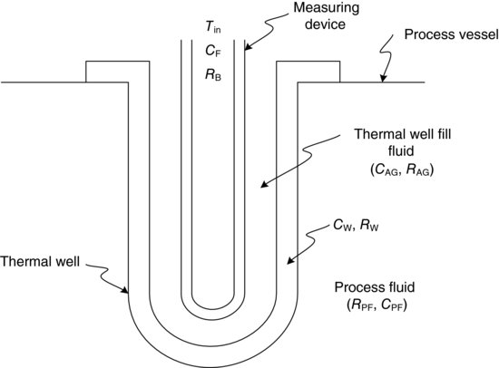
Every component in the measuring systems, as shown schematically in Figure 7.21, has an associated time constant, τ, where τ = RC (see Equation 3.28). So, each component in the measuring system will increase the measurement lag depending on the size of its time constant. Good practice dictates that the dominant time constant is the process fluid time constant, τPF = RPFCPF. The other time constants (thermal well, τw = RwCw; thermal well fluid, τAG = RAGCAG; and measuring device, τB = RBCF) should be as small as possible.

These time constants may be minimized in various ways. For instance, τw can be reduced by choosing a thermal well made from a material of low thermal resistance and also made as small as possible to reduce Cw. To minimize τAG, the air gap is filled with high thermally conductive fluid to decrease RAG or the measuring device is attached via welding to the well. Using the smallest bulb and shortest capillary possible to reduce both RB and CF will minimize τB. With respect to short capillary runs in a FTS to increase response speed a transmitter is mounted close to the process and a gas-filled bulb is used. This is done to minimize capillary length and gas is used because its thermal capacity, CF, is low. This in turn results in a small measurement time constant since the pressure signal from the FTS is changed to an electronic signal of 4–20 mA sooner without a long capillary run.

When using an RTD or a TC the time constant considerations are similar but the actual response times of the devices will vary. The FTS and RTD will have response times of nearly the same magnitude, while the TC is somewhat faster. For a TC, τB varies with the device's construction and length of the extension wires. Hence, a TC made of small wire with short extension wires will give a fast response. A typical TC response is around 0.5 seconds.

Let us put some numbers on the response times of the other two temperature measurement devices. The FTS and RTD have similar response times except that the response of the RTD in water is generally longer than the FTS due to its greater internal resistance. But for the same size bulb, either a liquid FTS or RTD has a time constant of about 3 seconds.

For an FTS the capillary has a time constant of 0.55 seconds per 10 feet, and thus it is obvious why a transmitter is often used since some capillaries can be up to 100 feet long. Using a short capillary, with a gas-filled system and a transmitter, results in a response that is two times faster than the liquid-filled system with a long capillary.

The response time of RTD or FTS bulbs in a thermal well depends on the material of the well and the clearance between the bulb and the well. For a bulb in a dry well a typical time constant is 1–2 minutes, while for a bulb with thermal fluid in the well the following apply:

• in a gas stream – τ is the same as for the dry well due to the high thermal resistance of the gas (τPF is very large).
• in a liquid stream – τ should be about two to three times that of the bulb alone, since the thermal resistance of the liquid is very small (τPF is very small) and the response improves with the lowering of the thermal well fluid resistance, that is, make τAG as small as possible.

If it is necessary to use a thick metal or ceramic well due to corrosive process fluid, the response time can increase to 10 times that of the bulb alone. In addition, a large well creates a static error as a result of conduction along the wall of the thermal well. The addition of a large well can increase the measuring device plus well time constant by approximately 1.5 minutes. This increase can be detrimental in certain processes, that is, exothermic reactor, but is not significant in others.

The following are general rules of thumb for reducing temperature measurement lag:

The whole point of the preceding discussion on minimizing temperature measurement lag in the temperature control loop is to make you aware that this is important in slow as well as fast loops.

7.5.1 The Endothermic Reactor Temperature Control Loop

A good example of an endothermic process is a process heat exchanger being used to heat a fluid from the inlet temperature, T1, to an outlet temperature, T2, as shown previously in Figure 6.2. This heat exchanger's response will be that of a single large dominant capacitance with at least 30 seconds of dead time. Typically either a PI or PID controller is used. Derivative action can be used since the temperature measurement is not noisy. The response of the loop under PID control will be equal to that of P-only control except the temperature will be maintained at the desired set point.

The steady-state gain of the heat exchanger is calculated from Equation 7.11:

(7.11)

The process gain, Kp, is a function of the load, Fw, as in the case of liquid level control previously discussed. However, Fw is not the only load; it is one of several. Other loads include the inlet and outlet temperatures of the cold fluid stream. The steady-state equation describing the behaviour of the heat exchanger is given by Equations 7.12 and 7.13:

(7.12)

(7.13)

where Cp is the specific heat of Fw; λ is the heat of condensation; Fw is the flow of cold fluid (load variable); T1 is the inlet temperature of cold fluid (load variable); and T2 is the outlet temperature of cold fluid (load variable).

The heat exchanger energy balance equation can be solved for the heat exchanger gain, Kp, as shown in Equation 7.14:

(7.14)

As expected the gain is inversely proportional to the load, Fw. This result is identical to that for the liquid level process and may be minimized with similar approaches.

A valve positioner, V/P, can also be added to the flow valve as described in the case of liquid level control. However, if there is a chance of a supply upset to the heat exchanger, a temperature on flow cascade is used instead, as shown in Figure 6.4. Another approach to minimizing supply upsets is to use a pressure regulator ahead of the steam. The pressure regulator is used to make the steam supply pressure constant. This scheme negates the need for another flow loop while still providing protection against supply upsets.

There are many methods used in controlling heat exchangers. Figures 7.22, 7.23, 7.24 and 7.25 show several methods in addition to the basic feedback loop, in which the flow of steam was directly throttled by the temperature controller.

Figure 7.22 Temperature control via level control (Courtesy of REM Technology Inc -Spartan Controls Ltd).

Figure 7.23 Control scheme for critical temperature control.

Figure 7.24 Variation of critical temperature control scheme.

Figure 7.25 Temperature control scheme for capacity-limited exchangers.

Figure 7.22 shows a situation in which Fs is a wild flow and T2 is controlled by controlling the condensate level in the heat exchanger, that is, overhead condenser. When the temperature is too high, the valve closes, which causes condensate to cover more tubes and reduce heat transfer to the cold fluid. Because the condensation time is large, the response is slower than for other systems. Also, due to condensate splash, T2 can show significant fluctuations.

Figure 7.23 shows a scheme employed when temperature control is critical and the response time, τ1, of the heat exchanger is very long.

In this approach a sidestream of the input Fw is bypassed and mixed with the outlet Fw. This gives fast response, with an energy penalty of first heating up and then cooling down Fw. It is also necessary to ensure good mixing at the output and to ensure a fast response in the temperature measurement, since a flow loop is being used. Another variation of the control scheme of Figure 7.23 is shown in Figure 7.24.

The scheme shown in Figure 7.24 provides control over a wider range of Fw and gives a nearly constant process gain. Hot and cold Fw are blended together to maintain a uniform T1. The energy penalty for this scheme is the cooling of the stream the energy of which has been expended in heating up.

The scheme shown in Figure 7.25 throttles Fw, to maintain T2, and is usually used in heat exchangers that are capacity limited. It is more important to maintain T2 at the set point than to maintain Fw at a given demand.

A detailed discussion of tube and shell, aerial coolers and fired heaters is found in the Hydrocarbon Processing articles by W.C. Driedger [9,10].

7.5.2 The Exothermic Reactor Temperature Control Loop

The exothermic reactor is perhaps the most difficult process to control due to its instability and extreme non-linear response [8]. A chemical reactor is quite often an exothermic process where some feedstock and catalyst are mixed together, and the temperature must be controlled at a specific set point. A typical temperature control scheme is illustrated in Figure 7.26.

Figure 7.26 Control scheme for an exothermic reactor.

The degree of stability that can be achieved in this temperature control loop depends on the rate at which the heat can be removed from the reactor. In other words, the reactor can be stabilized if the reaction temperature changes fairly slowly when compared to the rate at which the jacket temperature changes. The idea of the control loop shown in Figure 7.26 is that once the feedstock and catalyst are added, hot water in the jacket is used to initiate the reaction. As the reaction temperature increases, the controller output decreases, closing the hot water valve, which is air to open and opening the coldwater valve, which is air to close. A valve positioner, V/P, is used to minimize valve hysteresis. The pump and multiple water inputs to the jacket are used to minimize dead time and to change the jacket temperature as quickly as possible, that is, minimize the time constant of the jacket.

Typically a PID controller is used, but using a proportional-only controller may stabilize the reactor provided that the reactor is the dominant single capacitance in the loop and there is no appreciable dead time.3

Extremely fast reactions are sometimes carried out in semi-batch fashion to prevent a runaway temperature. In this case, one reagent is continuously added to a cooled reactor containing the other reagent or catalyst, and the addition rate is controlled to maintain a given batch temperature or a given heat removal rate. For safe operation, the temperature is kept high enough to ensure that a low concentration of the added reactant is required.

Often an emergency control system4 is implemented to stop the reaction by dumping the charge or stopping the catalyst flow in case the main control fails to halt a runaway reaction temperature. Other typical reactor control schemes can be found in References [3, 8].

In addition to these problems there is also the problem of the extreme non-linear process response. As before, the gain is a function of the temperature operating level. For the control system shown, the gain is defined by Equation 7.15:

(7.15)

In this equation, T is the reactor temperature and Fw is the cooling/heating water flow to the reactor jacket. Assuming perfect mixing in the reactor and a constant rate of heat evolution, the gain can be approximated as shown in Equation 7.16 where Q is the rate of heat generation:

(7.16)

Due to this non-linearity as well as to the problems mentioned earlier, some exothermic reactors are controlled with advanced control techniques such as feedforward, model reference or adaptive control [11].

7.6 Pump Control

The flow and pressure of streams discharging from pumps must be controlled. Throttling a discharge valve on a centrifugal pump and manipulating the recirculating valve on a reciprocating pump are both reasonable means of control. The most efficient control method is to use a variable speed motor to control the output of the pump [12].

7.7 Compressor Control

Simply stated, compressors are employed whenever a gas at a certain pressure in one location is required to be at a higher pressure at another location. However, this belies the fact that compressors are major ticket items in the capital cost of a chemical or petroleum plant. For example, a large centrifugal compressor with a gas turbine is an investment of many million dollars.

Two major types of compressors are commonly used in chemical and petroleum plants, reciprocating and centrifugal compressors.

7.7.1 Reciprocating Compressor Control

Control of reciprocating compressors [13] involves the control of compressor capacity, engine load and speed; the control of auxiliary items on the compressor package; and the control of compressor safety.

Control of Compressor Capacity, Engine Load and Speed

Compressor capacity is controlled by varying the driver speed, opening or closing fixed or variable volume clearance pockets, activating pneumatic suction valve unloaders, bypassing gas back to suction or varying suction pressure. Driver speed control is not always possible with synchronous AC motors although solid state devices are now available for varying input frequency and speed. There is not space and it is outside the scope of this book to go into the details of these electromechanical control mechanisms. The interested reader is directed to the Gas Processors Suppliers Association, Engineering Data Book [14].

Control of Auxiliary Items on the Compressor Package

Oil, water and gas temperatures, oil, water and scrubber liquid levels and fuel and starting gas pressures need to be controlled.

Control of Compressor Safety

Safety shutdown controls must also be provided in case of harmful temperatures, pressures, speed, vibration, engine load and liquid levels.

7.7.2 Centrifugal Compressor Control

As mentioned previously, a large centrifugal compressor with a gas turbine as a driver is typically a multi-million dollar investment. A dedicated computer control system is usually employed to monitor multiple operating parameters and that is specifically designed for the purpose. Such a control system is shown in Figure 7.27.

Figure 7.27 A REMVue Compressor Control Station (Courtesy of REM Technology Inc.-Spartan Controls Ltd.).

The control of a centrifugal compressor involves the control of capacity, the prevention of surge and the protection of equipment.

Capacity Control

The means available for controlling compressor capacity are suction throttling, discharge throttling, recirculation, variable guide vanes and motor speed control. Most of these controls are used in practice and which is best depends on the application. Some of the pros and cons of these alternative control methods are as follows:

Each of the methods of control affects the compressor curve to produce a set of curves called the compressor map (Figure 7.28).

Figure 7.28 A typical compressor map.

The various curves show the compressor characteristic at different values of the parameter being varied, such as inlet valve setting or speed. At each crossing of a compressor curve and a system curve, specific operating points occur which collectively establish the controllable range.

If the load on the compressor changes – that is the system curve changes – as shown in Figure 7.29, the operating point moves along the compressor curve. The range within the compressor curve is called the operating range (shown as points 1 to 2 in Figure 7.29).

Figure 7.29 Compressor load changes.

Returning to Figure 7.28 it can be seen that each compressor curve shows two end points. The lower right end point is relevant when discussing capacity control. Beyond the lower right end point the volume is so great that the internal flow velocity approaches sonic. A further drop in discharge pressure cannot affect the inlet flow therefore the flow rate no longer increases – this phenomenon is termed stonewalling.

Surge Prevention

Beyond the upper left end point of Figure 7.29, ΔP drops to a minimum and then rises again. This causes severe oscillations known as surge. As the pressure rises up the curve it eventually reaches a maximum. The pressure cannot fall unless some of the gas flows out of the discharge volume or into the inlet volume.

The symptoms of surge are pulsating pressure, rapid flow reversals, a drop in motor current and a jump in turbine speed. Continuous, rapid flow reversals can cause severe damage to the compressor. In axial compressors the blades may touch, resulting in instant destruction. However, centrifugal compressors are more rugged and only seal damage results [15].

The frequency of surge varies from 5 to 50 Hz. Suction and discharge volumes also influence surge. Minimizing the volume that has to be depressured can mitigate surge. Preventing ΔP from getting too high also prevents surge. Surge protection involves the determination of the surge limit line, that is, the limiting values of ΔP versus throughput that can initiate surge. Surge control keeps the compressor from crossing a surge control line that is arbitrarily set at a safe distance from the surge limit line [16].

The above compressor control theory is applied in the following example [15]. For more details on centrifugal compressors and their control, the interested reader is again directed to the Gas Processors Suppliers Association, Engineering Data Book [17] or the ISA Instructional Resource Package on Centrifugal and Axial Compressor Control [18].

Application Example

The application to be considered is a plant with a compressor drawing vapour from the top of a distillation column and moving this vapour to downstream processing units. The plant also has a considerable amount of waste heat in the form of steam, therefore, it is economically worthwhile to use steam turbines as drivers with superheated steam as the motive force. The schematic of the example plant is shown in Figure 7.30.

Figure 7.30 Compressor control example process schematic.

In order to control the compressor, its purpose in terms of a process variable needs to be known. The purpose of the compressor in this application example is to control the pressure at the top of the column. A suitable measuring instrument would be a pressure transmitter located at the knock out (KO) drum. The compressor throughput is controlled by speed control on the steam turbine. Steam turbines generally have special control valves that are an integral part of the machine and usually have their own governors. The pressure controller provides a set point for the governor.

Excess flow control (stonewall) protection is not needed as long as the compressor is not grossly oversized and the downstream process will provide sufficient backpressure to prevent excess flow. The process fluid is a light hydrocarbon and is never vented directly to atmosphere.

However, minimum flow (surge) protection is needed as every compressor needs surge protection. The surge loop is placed as close as possible to the discharge. A check valve is placed downstream of the recycle tee to prevent recycling the entire downstream process flow.

The recycle line returns to the suction KO drum. A cooler must also form a part of the recycle loop as there is no other way of removing the energy that accumulates as heat of compression.

In order to control surge the compressor map must be known. From the Fan laws we know that flow varies proportionally to speed and ΔP varies with speed squared:

(7.17)

(7.18)

From this we can calculate a family of curves based on the original compressor curve. These curves can be well fitted by a cubic equation. Surge occurs at the maximum or flat part of the curve. Applying the Fan laws and solving for the maxima result in a quadratic equation called the surge line. To avoid surge, the compressor never operates to the left of the surge line, so the square of the flow must be greater than proportionality constant times the ΔP:

(7.19)

In order to provide surge control, suction flow and ΔP must be measured. Suction flow must be in terms of actual, not standard volume units at the inlet. The effects causing surge are based on gas velocity, not mass flow. These measurements are made as follows. ΔP is measured across the compressor. A venturi, which has by definition output proportional to the square of the flow, is placed in the compressor suction. It is important that the flow transmitter not apply a square root to provide a linear signal so that it may be used directly in the surge controller without further squaring.

In order to apply these process measurements, the compressor map is cast into a new form, ΔP versus the square of the flow, which results in a straight line for the surge line. However, it is not a good idea to use the surge line as the set point to the surge controller because of instrument error, transmitter, controller and valve delays, compressor variations with time and molecular weight variations. Instead a surge control line is established perhaps 5% to the right of the actual surge line, as a safety factor.

The resulting, complete compressor control system with pressure/speed and surge loops is shown in Figure 7.31.

Figure 7.31 Complete compressor control system schematic.

As always, it is important to verify the control scheme dynamically with the use of a suitable dynamic simulator. Other application examples that are documented in the literature [11, 19, 20] include a substantial emphasis on the importance of dynamic simulation for control scheme design validation and performance evaluation.

Compressors' Performance Optimization with Air–Fuel Ratio and Slipstream Control

Compressors are powered by electric motors or reciprocating internal combustion engines (RICEs), which supply the load demanded by the compressor at the desired speed. RICEs require fuel flow control to achieve and maintain the desired speed. Speed is controlled by a governor that measures the rotational speed, compares to the desired speed and increases or decreases the fuel supplied to the engine. Electronic governors are replacing mechanical governors because of greater precision and reduced maintenance needs. In the electronic governor, the speed is measured by pulses generated in an induction coil or Hall-effect pickup by flywheel gear teeth or a flywheel stud. These pulses are converted to an analog signal. This analog signal is compared to an analog voltage proportional to the set point or desired speed by a PID (proportional, integral and derivative) software algorithm in the controller. If the engine speed is less than the set point speed, the PID analog output to a fuel valve actuator is increased to increase the fuel flow to the engine. The reverse occurs for an excess speed. The factors controlling the relative amounts of proportional, integral and derivative functions can be adjusted to ensure an optimum response to changes in compressor load or desired speed.

Air control is necessary for both spark-ignited (SI) engines and compression-ignited (CI) engines to achieve regulatory exhaust emissions control. In the past no air control was used for CI engines and a carburettor was commonly used for air to fuel ratio control. The advent of emissions regulations, particularly for oxides of nitrogen, NOx, has led to the predominant use of electronic control of the engine air. Emissions control can be very complex in detail. In summary, the amount of air supplied to the engine is controlled by a valve actuator. A software algorithm determines an air requirement according to the engine speed, load, air temperature and so on and provides an electrical signal to an air actuator. For many SI engines the NOx emissions are reduced in an exhaust catalyst. To ensure these catalysts achieve the desired emissions reductions, very precise control of the air to fuel ratio is required.

In the natural gas industry the majority of gas compressors are powered by SI RICEs with natural gas fuel. All gas compressors have leaks at rotational or sliding seals. In a novel control application, the natural gas from these leaks is collected and added to the engine air to supplement the normal engine fuel. Since the compressor leak rates are variable in time and magnitude, the addition of this gas to the engine air represents a control challenge. A commercial control system, known as SlipStream, is able to achieve the engine control necessary to both meet emissions regulations and save fuel costs.

7.8 Boiler Control

Boilers produce steam for power generation and heat, this is referred to as cogeneration. To control boilers, one requires complete combustion without too much excess air. The boiler's water level must be maintained by setting the feed water flow in equal to the steam flow rate out. The boiler must be able to control steam pressure and the temperature of superheated steam as demand fluctuates [12].

7.8.1 Combustion Control

The control scheme must burn all the fuel with minimal excess air. There is a risk of too little air, resulting in carbon monoxide production from partial combustion and excess fuel. This excess fuel is not only expensive, it is dangerous as it may explode if the air flow is increased. If there is too much air, the production of carbon monoxide is minimized. However, the excess air that is not used in combustion cools the flue gas, resulting in less efficient heat transfer to the boiler.

Optimally, the flue gas should be composed of 0.5–2% oxygen, and carbon monoxide production should remain in the parts per million, ppm [12]. These flue gas composition values depend on many variables, including the quality of fuel used, the boiler's condition and the steam demand in the plant.

For steady-state control the carbon monoxide and oxygen in the flue gas should be controlled.

For unsteady-state operation the control scheme is more complex. A high selector is used to set the set point on the airflow controller, and a low selector is used to control the ratio controller on the fuel side (Figure 7.32) [12]. For an increase in heat demand, the demand signal will be higher than either the fuel or air flow measurements. This will be passed by the high selector (>) to the airflow controller [12]. The increase in air flow will then be transferred through the low selector (<) to the ratio controller on the fuel side [12]. This ensures no excess in fuel since airflow leads fuel flow for an increase in steam demand.

Figure 7.32 Combustion control scheme.

When steam demand decreases, the demand signal will be passed via the low selector (<) to the fuel flow and the air flow will be lowered by the ratio controller. Air flow will lag fuel flow on a decrease in demand, ensuring no excess fuel build-up in the system [12].

7.8.2 Water Drum Level Control

To understand how to control the level in the water drum for the boiler, one must first understand the shrink–swell phenomena of this process unit. If the demand for steam increases, the pressure in the boiler decreases. Therefore, more water boils to steam and the vapour bubbles in the evaporator tubes increase in size. This expansion in bubble size and increase in boiled water lift more liquid into the water drum, increasing the level. As the drum level increases, a controller will add less feed water to compensate. However, this swell resulting from increased steam demand actually requires more feed water. To correct this error, a shrink–swell compensator can be used on the drum level measurement [12].

The shrink–swell compensator works by detecting that an increase in steam flow has occurred, corresponding to a decrease in pressure. Therefore a negative correction is applied to the level signal. As the swell subsides, the pressure increases and the corrective action is cancelled.

A decrease in steam flow would similarly result in a rising pressure. This increased pressure causes the water drum level to shrink, since apparent level decreases due to a smaller bubble size in the evaporating tubes. Once again the shrink–swell compensator would correct the response of the level controller for the water drum.

7.8.3 Water Drum Pressure Control

The pressure control system is used to maintain the energy within the boiler at a constant value. Pressure depends on the demand for steam in the plant and the rate of steam generation in the boiler.

To quantify the demand for steam in the plant, the controller relies on the steam flow and pressure. If the steam demand increases, the steam flow increases and the pressure decreases, calling for more generation of steam. This increase in firing rate demand increases the amount of fuel burned and maintains the thermal energy of the boiler during an increase in demand for steam.

7.8.4 Steam Temperature Control

Superheaters are used to raise the steam temperature above the saturation point to get superheated steam. As explained in Section 7.8.3, the firing rate of the boiler is controlled by steam demand in the plant. The heat generated in the boiler is first used in the evaporating tubes and then the superheating tubes.

So, if the demand for steam is low, there is a decrease in the boiler's firing rate and less energy is transferred to the superheaters. However, at high steam demand, more fuel is burned to increase the boiler's steam generation, making more energy available for the superheaters. Since the temperature of the superheated steam must be maintained at a constant value, feed water is added to keep the temperature from getting too high (Figure 7.33). Although this feed water will decrease boiler efficiency it is important for improved temperature control.

Figure 7.33 Control scheme for superheated steam.

Control must always be balanced to ensure safety and maximize benefits while minimizing losses.

References

1. Buckley, P.S. (1964) Techniques of Process Control, John Wiley & Sons, New York, p. 167.

2. Shinskey, F.G. (1997) Averaging level control. Chemical Processing, 60(9), 58.

3. Shinskey, F.G. (1967) Process Control Systems, McGraw-Hill, New York, p. 147.

4. Taylor, A.J. and La Grange, T.G. (2002) Optimize surge vessel control. Hydrocarbon Processing, 81(5), 49–52.

5. Åström, K.J. and Wittenmark, B. (1984) Computer Controlled Systems: Theory and Design, Prentice Hall, New Jersey, pp. 351–352.

6. Marlin, T.E. (1995) Process Control: Designing Processes and Control Systems for Dynamic Performance, McGraw-Hill, New York, pp. 538–540.

7. Ogunnaîke, B.A. and Ray, W.H. (1994) Process Dynamics, Modeling, and Control, Oxford University Press, New York, pp. 628–629.

8. Seborg, D.E., Edgar, T.F. and Mellichamp, D.A. (1989) Process Dynamics and Control, John Wiley & Sons, New York.

9. Driedger, W.C. (1997) Controlling fired heaters. Hydrocarbon Processing, April, 103–116.

10. Driedger, W.C. (1996) Controlling shell and tube exchangers. Hydrocarbon Processing, March, 111–132.

11. Muhrer, C.A., Collura, M.A. and Luyben, W.L. (1990) Control of vapour recompression distillation columns. Industrial and Engineering Chemistry Research, 29(1), 59–71.

12. Shinskey, F.G. (1996) Process Control Systems, 4th edn, McGraw-Hill, pp. 288–295.

13. Manning, F.S. and Thompson, R.E. (1995) Oil Field Processing, vol. 2, Chapter 15, PennWell Books, Tulsa, OK, USA, p. 340.

14. Gas Processors Suppliers Association (1998) Engineering Data Book, vol. I, 11th edn, GPSA, FPS Version, Section 13, pp. 14–21.

15. Driedger, W.C. (1998) Controlling Compressors. Lecture Notes, ENCH 529 Process Dynamics and Control, University of Calgary, March 16, 1998.

16. Magliozzi, T.L. (1967) Control system prevents surging in centrifugal-flow compressors. Chemical Engineering, May, 139–142.

17. Gas Processors Suppliers Association (1998) Engineering Data Book, vol. I, 11th edn, GPSA, FPS Version, Section 13, pp. 33–35.

18. McMillan, G.K. (1983) Centrifugal and Axial Compressor Control, Instrument Society of America, Research Triangle Park, NC, USA, pp. 57–74.

19. Campos, M.C.M.M. and Rodrigues, P.S.B. (1993) Practical control strategy eliminates FCCU compressor surge problems. Oil and Gas Journal, 91(2), 29–32.

20. Van der Wal, G., Haelsig, C.P. and Schulte, D. (1996/97) Minimising investment with dynamic simulation. Petroleum Technology Quarterly, Winter, 69–75.

1 Also called the quarter decay ratio (QDR), see Chapter 5 for more details.

2 For a direct acting controller, e = CV – SP.

3 Similar to a gas pressure loop.

4 Override controls.