6

Advanced Topics in Classical Automatic Control

Up to this point discussion has been restricted to feedback control loops, the most common control method used in process industries. However, there are a number of more complex control techniques that should also be considered [1], which can provide improved and economic process control. Some of the control schemes that are discussed in this chapter include cascade, feedforward, ratio and override control. These schemes are classified as ‘advanced classical’ [1] topics and are widely used in industry.

6.1 Cascade Control

Leading industrial practitioners have indicated that cascade control is a widely used controller configuration. Hence, it needs to be stressed in an undergraduate control course and its inclusion here is as the fore most advanced classical control technique.

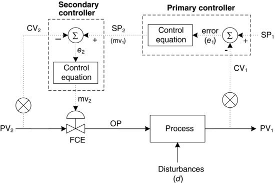
Cascade control is a control technique that uses two controllers with one feedback loop nested inside the other [2–4]. The output of the primary controller acts as the set point for the secondary controller. The secondary controller controls the final control element (FCE). A typical cascade control loop is illustrated in Figure 6.1.

Figure 6.1 Cascade control system.

To better understand cascade control, we will examine a typical feedback control scheme and consider how it may be improved through the use of cascade control. Let us consider the feedback control loop for a heat exchanger, shown in Figure 6.2.

Figure 6.2 Feedback control loop for a heat exchanger (steam supply loop).

In this example of a heat exchanger, the energy is provided by steam flow, Fs, and is used to heat an entering fluid, Fw, from an inlet temperature, T1, to an outlet temperature, T2. If the controller was properly tuned and there is a change in Fw, the change in T2 will be sensed and the temperature controller will then change its output by repositioning the valve to bring the outlet temperature back to the set point. In other words, the controller moves the variance from one stream to another and thus mitigates changes in the process variable, PV.

Let us now consider another possible type of upset: a supply side upset. If the steam, Fs, is coming from a supply header which is also servicing other users, there is a possibility that as the other users' needs vary, pressure upsets will occur causing changes in the steam supply Fs. Suppose that another user demanded steam quantities that caused a pressure drop in the header, thus resulting in a drop in steam flow to the exchanger. The only way this drop in Fs could be measured would be as a drop in the outlet temperature, T2. This deviation from set point would be sensed and compensated for in the same manner as for the stream load upset, Fw. The response of the process variable, T2, to the two situations is shown in Figure 6.3.

Figure 6.3 Heat exchanger outlet temperature response.

In both cases the process variable, T2, would dampen out in the period, τn. However, for the supply upset situation the feedback control may cause the temperature to be in a constant state of flux. For instance, if the valve (when open to 50%) supplies the needed amount of steam, the outlet temperature will be at the set point. However, the flow through the valve is a function of the pressure drop across it. Therefore, if there is a decrease in inlet pressure the flow will decrease, even though the valve is 50% open. This disturbance will propagate through the dead time and capacitive lag of the heat exchanger before it emerges as an outlet temperature deviation, at which time the necessary control action will be taken to bring the temperature back to the set point. The response will damp out with a period, τn, back to the set point. If τn were a minute or two or even longer, the process might be in a constant state of flux and never settle to the desired set point.

The problem is that the controller output sets a valve opening rather than setting an energy supply requirement. With a constant pressure drop across the valve, the relationship between valve position and steam flow is constant, but if the pressure drop changes this relationship changes. Thus, it is better to set the steam requirement rather than valve position. As long as the valve can supply the energy requirement, it does not matter how wide open the valve is, only how much energy is being delivered. Hence, for this process better control can be achieved by using cascade control.

Now we will apply cascade control to the same heat exchanger to control supply side upsets. In Figure 6.4, the temperature loop (primary loop or master) is used to adjust the set point of the flow control loop (secondary loop or slave).

Figure 6.4 Typical cascade control loop for a heat exchanger.

With cascade control in place, if a set point change is made in the temperature controller, or if a load upset occurs that changes Fw, the output of the temperature controller will change the steam flow controller set point. The flow loop operates so much faster than the temperature loop that the temperature controller does not in fact know whether its output is going directly to a valve or as a set point to another controller. In general, the control loop closest to the controlled variable is called the primary, outer or master loop. The control loop closest to the supply to the process is called the secondary, inner or slave loop. In the heat exchanger example given, the temperature loop is the primary loop and the flow loop is the secondary loop.

Both the primary and secondary loops have their own response period, independent of whether they are in a cascade configuration or not. The response period of the primary loop is τ1 and that of the secondary loop is τ2. In order that cascade control works effectively, τ1 ≥ 4τ2. What this rule of thumb implies is that the primary loop should never know that there is a secondary loop. The secondary loop should be able to respond as quickly as the FCE. If this rule is followed then there will be little interaction between the two loops and the control scheme will function normally.

6.1.1 Starting up a Cascade System

To put a cascade system into operation

Note: When tuning the primary controller there should be no interaction between the primary and secondary loops. If there is, it means that the primary loop is not slow enough in comparison to the secondary.

One of the most common forms of cascade is the output of a primary controller acting as a set point to a valve positioner. Other common industrial examples of cascade control include level to flow cascade control, heat exchanger temperature control as per the example above, temperature control of furnaces/fired heaters, temperature control of exothermic stirred chemical reactors and distillation composition to temperature to flow cascade control. Most modern advanced process control schemes such as model predictive control are also implemented in a cascade arrangement over a regulatory control layer.

6.2 Feedforward Control

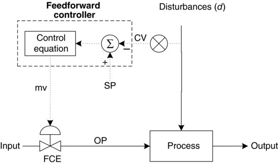
One of the disadvantages to using feedback control is that a disturbance must propagate through the process before it is detected and action is taken to correct it. This type of control is sufficient for processes in which some deviation from the set point is acceptable. However, there are certain processes where this set point deviation must be minimized. Feedforward control can accomplish this because it corrects and/or minimizes disturbances before they enter the process [3,4]. A typical feedforward control system is shown in Figure 6.5.

Figure 6.5 Feedforward control system.

In its simplest form, a feedforward controller merely proportions the corrective action to the size of the disturbance. In other words, the control equation is merely a gain based on steady state, that is, mass or energy balance at steady state. This does not take into account any of the process dynamics of the system. If there is a difference, or lag, in the speed of the process response to the control action when compared to that of the disturbance, it may be necessary to introduce some dynamic compensation into the control equation. The dynamic compensation correctly times the control action and response thus giving increased accuracy in the feedforward control.

In general, the feedforward dynamic elements will not be physically realizable. In other words, they cannot be implemented exactly. For instance, if the process disturbance measurement contains dead time, or lag, the feedforward dynamic compensation would have to be a predictor, which of course is impossible unless an exact and very fast dynamic model of the process is available. In practice, the feedforward dynamic elements are approximated by a lead lag network [3,4] that is adjusted to yield as much disturbance rejection as possible over as wide a range as possible.

When feedforward control is used equations are needed to calculate the amount of the manipulated variable needed in order to compensate for the disturbance. This sounds simple enough; however, the equations must incorporate an understanding of the exact effect of the disturbances on the process variable. Therefore, one disadvantage of feedforward control is that the controllers often require sophisticated calculations as even steady models can be nonlinear and thus need more technical and engineering expertise in their implementation.

Another disadvantage of feedforward control is that all of the possible disturbances and their effects on the process must be precisely known. If unexpected disturbances enter the process when only feedforward control is used, no corrective action is taken and the errors will build up in the system. If all the disturbances were measurable and their effects on the process precisely known, a feedback control system for regulatory purposes would not be needed. However, such complete and error-free knowledge is never available, so feedforward is generally combined with feedback, as illustrated in Figure 6.6. The intent of this union is that the feedforward mitigates most of the effects of the principal disturbances and the feedback loops provide residual control and set point tracking.

Figure 6.6 Feedforward/feedback control system.

Consider the following example of the feedforward control of a heat exchanger with cascaded feedback trim control (shown in Figure 6.7). The addition of feedback and cascade control serves to eliminate offset due to modelling inaccuracies and other non-measured disturbances.

Figure 6.7 Combined feedforward and cascade control of a heat exchanger.

At steady state an overall heat balance can be written for the process as shown in Equations 6.1, 6.2 and 6.3:

(6.1)

(6.2)

Or

(6.3)

where λ is the enthalpy transferred by the steam condensing to form condensate (kJ/kg) and Cp is the heat capacity of the process fluid (kJ/kg K).

In this example, the inlet flow of liquid, W, and the temperature, T1, are measured to determine the amount of steam required as per Equation 6.3. The desired outlet temperature, T2, is the set point into the feedforward controller. The feedback temperature controller on the liquid stream measures T2 to adjust for any disturbances that are not corrected by the feedforward controller.

Typical response curves for a load upset would appear as shown in Figure 6.8. Included in this figure for comparison is the response curve for feedback control only (with a PID controller) on the same process.

Figure 6.8 Typical responses of the heat exchanger.

The response of the outlet temperature, T2, for the base case of the feedback control shows the type of improvement in control that can be achieved with even a simple steady-state feedforward controller. The lead/lag dynamic compensation [3,4] shows further improvement over the steady-state feedforward control.

Common industrial examples of feedforward control in addition to heat exchanger control as shown above include control of fired heaters, chemical reactors and distillation columns. Other examples include control of biological process systems, such as fermentors and activated sludge processes and so on. An industrial illustration of when feedforward control was combined with feedback to control dissolved oxygen addition to a municipal wastewater treatment process resulted in significant savings in air blower energy consumption for the wastewater treatment plant [5]. Figure 6.9 illustrates the successful control scheme.

Figure 6.9 Feedforward/feedback control of a wastewater denitrification process.

6.3 Ratio Control

Ratio control involves keeping the ratio between two variables fixed [2,4], as illustrated in Figure 6.9. Typically, these two variables, y and yw, are flow rates, where yw is the wild or uncontrolled flow rate and y is the manipulated or controlled flow rate. The wild flow rate is measured, and the controlled flow rate is then adjusted to maintain a fixed ratio between the two.

Ratio control can be considered a form of feedforward control. This is obviously true since in ratio control the process variable is measured upstream of the process, as is the case in feedforward control (Figure 6.4). Take, for example, a reactor with two liquid feed streams. Ratio control would ensure that these streams were being stoichiometrically fed to the reactor by measuring the flow of one stream and adjusting the other accordingly. The product stream would be of no real use in determining whether the stoichiometric ratio was met.

There are two methods by which the ratio between the two variables can be fixed when only one stream is being manipulated. The first is shown in Figure 6.10.

Figure 6.10 Typical ratio control system.

In this first scheme, both flows are measured and divided to obtain the actual ratio. This is then compared to the set point and the flow of y is adjusted based on the difference. The set point to the ratio controller is the desired ratio.

In the scheme shown in Figure 6.11, the flow of the wild stream, yw, is measured and then multiplied by the desired ratio. The output from the multiplier is the set point for the controller, which compares it to the measured flow and adjusts the flow of y accordingly. In this scenario, the desired ratio is a constant variable in the multiplier and if a new value for the ratio is needed, it must be set in the multiplier.

Figure 6.11 Typical ratio control system.

The ratio control configuration shown in Figure 6.10 will not have a steady loop gain because the ratio calculation itself is in the loop. The loop in Figure 6.10 may become nonlinear, making the control configuration in Figure 6.11 a more reliable model, since its loop gain is constant.

A common example of ratio control is the case of an adsorption column where a fixed ratio of V/L is desired. The wild flow rate is the vapour feed to the column, V, while the controlled flow rate is the liquid flow rate, L. The ratio control seeks to maintain constant absorption factors in the column by keeping a constant V/L profile.

6.4 Override Control (Auto Selectors)

Frequently a situation is encountered where two or more variables must not be allowed to exceed specified limits for reasons of economy, efficiency or safety. If the number of controlled variables is greater than the number of manipulated variables, a selection must be made for control purposes (single input/single output). A selector is used to accomplish this. Selectors are available in both electronic and pneumatic versions. The only difference between selectors is the number of inputs a particular hardware implementation may be able to accommodate. In this section specific examples of such selectors will be discussed. It must be kept in mind that these are only a few examples of such auto selectors [4].

The two basic building blocks for selector systems are the high and the low selector. The high selector, shown in Figure 6.12, will pass the highest value of the multiple inputs to the output signal, ignoring all other inputs.

Figure 6.12 High selector.

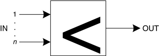
The low selector, shown in Figure 6.13, will choose the lowest of inputs to pass through as the output while ignoring all other inputs.

Figure 6.13 Low selector.

By using combinations of these basic building blocks it is possible to build other types of selectors, such as a median value selection, shown in Figure 6.14. The selector output for a median value selector is a signal that falls between the highest and lowest input.

Figure 6.14 Median value selector.

Let us investigate some typical applications of these selectors in four areas:

6.4.1 Protection of Equipment

To illustrate how selectors can be used to protect equipment, examine the pump system shown in Figure 6.15. The pump system demonstrates a situation where there are multiple measurements, multiple controllers and only one manipulated variable that can provide the following protection:

• Surge protection: when Pin drops below a certain minimum value, close the valve.
• High temperature: when the temperature of the pump exceeds a certain maximum temperature, close the valve.
• Excessive downstream pressure: when Po exceeds a certain maximum pressure, close the valve. (Assume Po > P shut off).

Figure 6.15 Protection of equipment – pump.

Surge Protection

As Pin begins to drop, the output, m1, will also decrease (note Increase/Increase action on pressure controller). The output, m1, will be selected by the first and second low selector and will be passed through as the manipulated variable causing the valve to close.

High Temperature and Excessive Downstream Pressure

If either the pump temperature or outlet pressure begins to increase, both outputs m2 and m3 begin to decrease (note Increase/Decrease action on both of these controllers). The smallest value will be chosen and passed through to manipulate the valve. In general, the smallest output from either of the controllers will always be operating the valve.

6.4.2 Auctioneering

The objective of auctioneering is to protect against the highest temperature sensed by one of many temperature transmitters. In the example shown in Figure 6.16, the control equipment consists of one controller, four transmitters and one FCE. The highest temperature will be selected by the high selectors and will be used as the measurement for controlling the fuel to the oven.

Figure 6.16 Auctioneering – temperature control in an oven.

6.4.3 Redundant Instrumentation

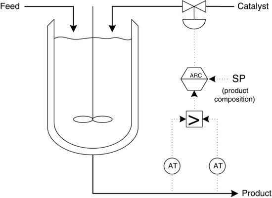
For an exothermic reactor (shown in Figure 6.17) too much catalyst can prove disastrous. By implementing a fail-safe scheme that consists of two composition transmitters that are analysers and a high selector, the highest reading from the analysers will be utilized by the composition controller to control catalyst flow. The following actions will occur in the event of catastrophic failure of the analysers:

Figure 6.17 Redundant instrumentation – reactor.

An alternate scheme, shown in Figure 6.18, implements analysers with a medium selector that will keep the process operating regardless of the failure mode of one of the analysers. The measurement variable to the controller will always be the median transmitter output. If one of the analysers fails, either upscale or downscale, the selector will still choose the median value.

Figure 6.18 Redundant instrument – reactor/median selector.

In summary, the amount or quantity of redundancy depends on the importance of the process unit (reactor, distillation column, etc.). This is because the higher the quantity of redundancy the higher the cost (capital/operating) becomes and, therefore, the economics must be justified.

6.4.4 Artificial Measurements

Some processes require certain operating constraints to be set. These are referred to as artificial measurements. These operating constraints can be set through the use of selectors. For example, consider a distillation column whose feed versus steam characteristic is shown in Figure 6.19.

Figure 6.19 Feed/steam characteristic of a distillation column.

Instead of operating the steam versus feed flow on a straight line, operating constraints are set. The operating constraints require a minimum steam rate of 10%, even if the feed rate drops to zero. This sets the low limit of the steam flow. Furthermore, at maximum feed rate the steam rate should not exceed a maximum flow of 90%, the high limit. These constraints can be implemented as shown in Figure 6.20.

Figure 6.20 Artificial constraints.

If the feed flow is within the safe operating region, the signal from the multiplier will pass through the high selector since it is higher than the low limit. It will also pass through the low selector since it is lower than the high limit, and then act as the set point for the steam flow controller. If the feed signal falls below the low limit or above the high limit the proper limit will be selected and that limit will be a constant high or low signal to the steam flow controller. This prevents the high and low limits from being exceeded.

6.5 Split Range Control

Split range control may be useful in processes where there is one controlled variable and there are extra manipulated variables. Each of the extra manipulated variables must be able to affect the controlled variable. An example of split range control is illustrated in the control of an exothermic reactor, Figure 6.21, which will also be discussed in further detail in Chapter 7 when we deal with reactor control more comprehensively.

Figure 6.21 Control scheme for an exothermic reactor.

The exothermic reactor in Figure 6.21 can be stabilized if the reaction temperature changes fairly slowly when compared to the rate at which the jacket temperature changes. The idea of the split range control loop shown in Figure 6.21 is that once the feedstock and catalyst are added, hot water in the jacket is used to initiate the reaction. As the reaction temperature increases, the controller output decreases, closing the hot water valve, which is air to open, and opening the cold water valve, which is air to close. This is split range control.

It is important to note that there are several implementation issues when applying split range control. One issue is the tuning of the system. When a different manipulated variable is selected by the controller, the closed loop process dynamics may change. Therefore the controller tuning should remain the same only if the process dynamics remain the same. For the example in Figure 6.21, this would mean that the hot water dynamics would be similar to the cold water dynamics. If the closed loop dynamics are significantly different, the controller tuning should be automatically changed, that is, a different set of tuning parameters should be used.

In practice there is a limit on how accurately a control valve can be adjusted. This has implications for the number of manipulated variables that may be used in split range. Split range control is normally limited to two or three manipulated variables for this reason. As a further consequence of inaccurate valves a split range control system could cycle if there is a dead band in which neither manipulated variable is adjusted. Valves in split range control systems are therefore calibrated to have an overlap, for example, of 10% to prevent this from occurring.

References

1. Seborg, D.E. (1984) A perspective on advanced strategies for process control. Modeling, Identification and Control, 15(3), 179–189.

2. Eckman, D.P. (1945) Principles of Industrial Process Control, John Wiley & Sons, New York (Metered and Ratio Control, pp. 194–199).

3. Murril, P.W. (1967) Automatic Control of Processes, International Textbook Company, Scranton, PA (Cascade/Ratio, pp. 431–444, Feedforward Control, pp. 405–425).

4. Shinskey, F.G. (1967) Process Control Systems, McGraw-Hill, New York (Cascade/Ratio, pp. 154–160, Feedforward Control, pp. 204–229, Override Control, pp. 167–169).

5. Young, B.R., Board, T. and Mormede, S. (2006) Advanced regulatory control of wastewater de-nitrification. Electrical & Automation Technology, August/September, 39–40.