
Workshop 6
Topics in Advanced Control
Theory without experience is sterile, practice without theory is blind.
—George Jay Anyon
Introduction
Prior to attempting this workshop, you should review Chapters 6 and 7 in the book.
This workshop will show how the response of feedback control (FBC) loops can be improved through the use of other control methods. These other methods include measuring common disturbances and taking action before they affect the controlled variable (feedforward control) and using a faster responding loop to decrease the response time of a system with a large time constant (cascade control). You will determine what conditions are necessary for feedforward or cascade control to be useful and identify which parameters reduce the effectiveness of these control methods.
Key Learning Objectives
Feedforward Control
Cascade Control
Ratio Control
Tasks
1. Basic Process Configuration
Build the system shown in Figure 6.1 using the Wilson package. The feed is pure water with a temperature of 20°C, atmospheric pressure and a flow rate of 1.5 m3/h. The outlet temperature of the heater should be set to 55°C with steam as the heating medium. Assume that the pressure drop is negligible, that is, set equal to zero. Incorporate dead time into the process by adding a pipe segment with a length of 1.0 m, a total volume of 0.2 m3 and a pressure drop of 0 kPa. Finally, add a separator with a volume of 1.2 m3 and set the liquid level set point at 50%. Alternatively, you might be able to modify the simulation you used for Workshop 4.
Figure 6.1 Simple heating system.

Use strip charts to view your results, monitoring the following variables: feed temperature, product temperature, steam heat flow, product molar flow. Select suitable ranges for each variable and iconize the strip chart view for later use.
Add two controllers to the system to set up FBC of the process:
Make sure that you correctly specify whether your controllers are direct acting or reverse acting. Set both controllers to automatic.
Finally add feed noise to the system using the Selector Block unit operation. The selector block is connected to the feed temperature. Create sine wave noise with an amplitude of 10°C and a period of 10 minutes. The feed temperature should still oscillate around a mean of 20°C.
2. Determine Base-Line Control Performance
The heater–tank system, shown in Figure 6.1, has a large capacitance, which should provide good attenuation of process disturbances and help reject high-frequency process noise. However, it will make the system slow to respond to set point changes or permanent disturbances, that is, feed rate changes. The significant dead time in the system will compound any control problems and make it difficult to achieve tight control of the system when only FBC is used.
- Vary the period of the disturbance to the feed temperature and fill in Table 6.1 to demonstrate this characteristic of the system.
- Should the magnitude of the feed temperature disturbance affect the attenuation?
- From your results, identify any deficiencies of the FBC system simulated above. If necessary, vary the temperature controller tuning constants to try to improve the performance of the control loop.
[Hint: How long does it take the controller to respond to a change in the feed temperature? Can the warm water temperature be stabilized by manipulating the tuning constants? How does the controller respond to changes in the feed rate, that is, step response testing?]
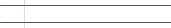
Table 6.1 Base-line control performance.

3. Feedforward Control
Feedforward control can be used to combat the control problems associated with processes containing significant dead time. This is achieved by measuring process disturbances and compensating for them before they affect the controlled variables. Ideal feedforward control is realized if pre-emptive control action is taken to completely cancel out the effect of measured disturbances before they enter the process. Sometimes the ideal feedforward controller is not realizable because disturbances affect the system more quickly than the manipulated variable. However, feedforward control can still be useful in these scenarios when teamed with FBC because the feedforward control reduces the duty on the master controller and improves the overall system response. Clearly, no action can be taken if the disturbances are not sensed or measured.
Build a feedforward controller for the heater–tank system, using the built-in process calculator function in VMGSim, to compensate for changes in the feed temperature before they become apparent in the warm water temperature. This feedforward control will be combined with the FBC to see if process response can be improved.
In order to obtain the actual feedback duty directly from the TIC-100 controller, create a fake heater with two fake streams (you can input the stream specifications as you like) and connect to the output of TIC-100 controller. If you are interested, you can find other ways to obtain the feedback duty without creating the fake heater.
Set up the following titles in cells Al–A6:
| Al | Actual Feed Temp |
| A2 | Nominal Feed Temp |
| A3 | Temp Difference |
| A4 | Process Gain 2 |
| A5 | Steam Valve Span |
| A6 | Process Gain 1 |
| A7 | Feedforward Duty |
| A8 | Feedback Duty |
| A9 | Total Duty |
Complete the spreadsheet as follows:
| B1 | Import the feed temperature from the process feed stream. |
| B2 | Import the nominal feed temperature which is equivalent to the feed temperature set point. [Hint: Refer to the Transfer Function operation.] |
| B3 | =B2–B1 |
| B4 | Input the value of the process gain between the product temperature and the feed temperature. [Hint: How much does the product temperature rise for a 1°C step increase in the feed temperature?] |
| B5 | Connect to the span of the heater duty valve. |
| B6 | Input the value of the process gain between the product temperature and the heater duty. [Hint: How much does the warm water temperature rise if the heater duty changes from 0% to 100%?] |
| B7 | The feedforward duty can be calculated from Equation 6.1. Incorporate this equation into the spreadsheet. |
where ΔQ represents the changes in heater duty required to produce 1°C change in the product temperature; ΔT is Nominal Feed Temperature – Actual Feed Temperature; Kp1 is Process Gain 1 between the product temperature and the feed temperature; SVSpan is Steam Valve Span; Kp2 is Process Gain 2 between the product temperature and the heater duty.
| B8 | Import the heat duty from the fake heater. |
| B9 | Add the FF duty from cell B7 to the FB duty from cell B8. |
Equation 6.1 is not necessarily exact at all values of the feed temperature due to the process non-linearity. An exact expression is not necessary for successful feedforward control; even if the calculated duty is incorrect by 50%, the controller will still perform better than with no feedforward action.
Export the result in cell B9 to the heater duty port. Your process should be similar to the one shown in Figure 6.2.
- Test the feedforward controller for the same range of feed temperature disturbances that you analysed for FBC in the previous task. (Due to the complexity of the feedforward controller designing, you might observe minor offset between the set point and PV in this case. If you are interested, verify the reason and find a solution to solve the offset problem.) Record the results in Table 6.2.
- How effective is the feedforward controller? What are its major deficiencies?
[Hint: Test the effectiveness of the feedforward controller for changes in the feed rate.] - Briefly comment on any implementation issues that might be relevant with feedforward control.
[Hint: How is the feedforward gain calculated? How can dynamics be incorporated into the feedforward controller? How important is tuning of the feedforward controller?]
Table 6.2 Feedforward control performance.
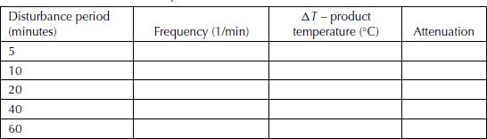
Figure 6.2 Feedforward control system.

4. Cascade Control
Cascade control is an alternative way to manage processes that contain large time constants and/or significant dead time. It is not necessary to sense or measure disturbances but a secondary variable must exist that directly affects the primary (master) loop and responds faster than the primary loop. The secondary variable is usually, but not necessarily always, a flow or a pressure that is directly controlled via a control valve. Normally, this secondary (slave) controller is a flow controller, a pressure controller or a fast-responding temperature controller. The time constant of the slave loop should be less than 25% of the time constant of the master loop for cascade control to be effective. Also, the secondary loop should contain little or no dead time. This allows the secondary variable to be controlled tightly, which provides attenuation for the primary loop.
Build a cascade controller for the heater–tank system using an inner loop that manipulates the steam rate based on the heater outlet (‘hot feed’) temperature. The master controller (separator temperature) should provide the set point for the slave loop and the slave controller should manipulate the steam rate directly. The process is shown in Figure 6.3.
Figure 6.3 Cascade control system.

To implement cascade control into your existing simulation, delete the feedforward controller but retain the separator level controller and the original separator temperature controller. The separator temperature controller will now be the master controller for the cascade loop.
Add another controller unit operation to the flow sheet. Connect the PV point to the ‘hot feed’ temperature. Connect the OP point to the heater energy stream (‘steam’) and specify ‘Direct Q’ between 0 and 5 × 10⁵ kJ/h. Connect the SP point (cascaded set point source) to the PV point of the master controller. Configure the controller mode to ‘cascade’ for the slave controller otherwise it will not work properly. The slave loop should be tuned tightly; specify a gain of 5 and an integral time of 10 minutes. The master loop can be tuned more loosely; specify a gain of 1.0 and an integral time of 10 minutes. Note that the gain of the master loop is not numerically comparable to the gain of the temperature loop from the previous simulation (without cascade control) because a different variable is being manipulated in the two cases. Your process should now be similar to the one shown in Figure 6.3.
- Test the cascade controller for the same range of feed temperature disturbances that you analysed for the previous two systems, which contained FBC only and feedforward control. Record the results in Table 6.3.
- Try varying the tuning constants for both the slave loop and the master loop. Which combination(s) of tuning constants work best?
- What comments can you make about the slave and master controller settings? How sensitive is the overall control performance to the slave loop tuning?
- Overall, how effective is the cascade controller?
[Hint: How does the controller respond to changes in the feed rate? How does the controller respond to changes in the master controller set point? Does the duty control valve open and shut excessively, that is, is there too much control action?] - What are the major advantages and shortcomings of cascade control?
- How does cascade control compare with feedforward control?
Table 6.3 Cascade control performance.

5. Ratio Control
Ratio control is a simple form of feedforward control that is commonly employed in controlling reactor feed compositions and in blending operations. It is also used to control the fuel to air ratio in heaters and boilers and to control the reflux ratio in distillation columns. The flow rate of one stream is used to provide the set point for another stream so that the ratio of the two streams is kept constant even if the flow of the first stream varies. Alternatively, the actual ratio between two flows can be used as the input to a controller.
Build a new system consisting of two streams, two separators and a mixer using the Wilson thermodynamic package. Pick any two components that are at liquid phase at ambient temperatures. The first stream should be pure component ‘A’ at 25°C and 100 kPa. The second stream should be pure component ‘B’ at the same temperature and pressure. Set the flow of the first stream to 400 kg/h and the second stream to 100 kg/h. These flows are consistent with the desired ratio of 4:1 between components A and B. The separators are used to simulate dead time in the system so choose relatively small volumes for the separators and locate them in series with the first stream. Both separators should be on level control rather than liquid flow control. Beware of the CV value of both control valves. Simulate process noise with a sine wave input to the first stream using an amplitude of 50 kg/h and a period of 10 minutes. The system should resemble the one shown in Figure 6.4.
Figure 6.4 Ratio control system.

Incorporate ratio control via a process calculator. Import the flow on the first stream into cell Al. Put the ratio of 0.25 in cell A2 and add a formula to give the flow of the second stream in cell A3. Export the results of cell A3 to the mass flow of the second stream.
Run the simulation in dynamic mode with several values of disturbance period. Watch how the combined flow rate and concentration in the product stream changes with different conditions. You may need to reduce the integrator step size to see the effects of very high frequency disturbances (period > 5 minutes).
- How effective is the ratio controller at filtering out low-frequency noise?
- How effective is the ratio controller at filtering out high-frequency noise?
- What are some of the advantages and limitations of ratio control?
- What is the significance of the dead time in the system?
[Hint: How would your answers change to the above questions if the dead time was the same for both streams?]
Present your findings on CD, DVD or thumb drive in a short report using MS-Word. Also include on the submitted media a copy of the VMGSim files which you used to generate your findings.