
Workshop 7
Distillation Control
Have confidence that if you have done a little thing well, you can do a bigger thing well, too.
—Joseph Storey
Introduction
Prior to attempting this workshop, you should review Chapter 8 in the book.
Distillation is one of the most important unit operations in chemical engineering. It forms the basis of many processes and is an essential part of many others. It presents a more difficult control problem compared with many other unit operations as at least five variables need to be controlled simultaneously and there are at least five variables available for manipulation. Thus a distillation column provides an example of a multiple-input multiple-output (MIMO) control problem. It is critical that variable pairing is done appropriately between controlled variables and manipulated variables. The overall control problem can usually be reduced to a 2 × 2 composition control problem since the inventory and pressure loops frequently do not interact with the composition loops. This workshop will highlight some fundamental rules of distillation control and show how a basic distillation control scheme can be selected.
Key Learning Objectives
Tasks
1. Basic Process Configuration
The distillation column shown in Figure 7.1 is typical of a stabilizer, which is found in most refineries. The column is designed to remove volatile components from potential gasoline blendstocks. The feed is usually a mixture of C3, C4 and C5. In this case, the feed contains 5% propane, 40% isobutane, 40% n-butane and 15% isopentane. The total flow rate is 40 000 bbl/day at 720 kPa and 30°C.
Figure 7.1 Stabilizer.
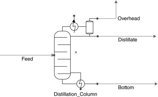
Use the Advanced Peng–Robinson property package and the above information to build a steady-state simulation model of the distillation column. The column contains 20 trays and a total condenser (a condenser vapour rate spec value of 0 can be used to simulate a total condenser). Feed enters at tray 10. The normal column overhead pressure is 700 kPa and there is a 20 kPa pressure difference that is evenly distributed between the condenser and the reboiler. Under steady-state design, size the distillation column using the ‘tower sizing’ function, enter the weir height as 10 cm and tray spacing as 60 cm, select the column type as ‘GlitschValve’, then run the ‘auto section design’. The automatic design result will be shown at the bottom and you will need these values in the dynamic model design. Your sizing result should look like this:

Make three specifications for all three degrees of freedom at the ‘Spec/Estimate’ tab, which are the flow of condenser vapour stream is 0, the C3 fraction of bottoms product is 0.01 wt% and the column is operating with a reflux ratio of 1.0.
View the results to get a feel of the column in steady-state mode.
[Hint: As VMGSim only have distillation columns with a partial condenser, the third degree of freedom in steady state is to set the overhead flow of the condenser as zero.]
Investigate the steady-state model and try to find out the answer for the below questions:
- How to obtain the reflux ratio, reboil ratio, reflux flow rate and reboil flow rate in your steady-state model?
- How much is the value for the condenser duty and reboiler duty?
- What is the temperature and pressure on trays 1, 5, 10, 15 and 20?
Note down all these values as they are the baseline and will be useful in later tasks.
2. Distillation Control Design via Steady-State Analysis
Ultimately the importance of process control is seen through increased overall process efficiency allowing the plant engineer to get the most from the process design. This is especially true of distillation control. Most distillation columns are inherently flexible and a wide range of product yields and compositions can be obtained at varying levels of energy input. A key requirement of any control system is that it relates directly to the process objectives. A control system that does not meet the process objectives or produces results that conflict with the process objectives does not add value to the process.
The first step of control system design is to identify the process objectives, which may not always be obvious. One process objective of the system shown in Figure 7.1 is to control the propane content of the bottoms at 0.01 wt%. However, other process objectives are not clear from the information given above. Controlling the reflux ratio at 1.0 may be desirable for the given conditions, but this is not a key process objective as it does not directly fix any property of the products or the energy consumption.
Some possible process objectives for this system include
- Minimum energy input,
- Maximum product yield,
- Minimum isopentane in the overhead product,
- Maximum recovery of C4+ components and
- Overhead temperature to meet utility requirement.
How many process objectives can be met simultaneously by the control system? A simple distillation column with no side draws and a total condenser has five degrees of freedom. A partial condenser (where there are two overhead products) adds one extra degree of freedom, as does each side draw. The degrees of freedom correspond to the number of control valves in the system:
- Distillate flow,
- Bottoms flow,
- Reflux flow,
- Cooling medium to the condenser (condenser duty),
- Heating medium to the reboiler (reboiler duty),
Three inventory/capacity variables must always be controlled in distillation:
One control valve (or degree of freedom) must be used for each controlled variable. This relationship between controlled variables and degrees of freedom (or control valves or manipulated variables) is known as variable pairing and is an important concept in control system design.
After the inventory and capacity variables are controlled, two further controlled variables can be fixed by the control system. In the stabilizer discussed above, we have already noted that we would like to control the propane content of the bottoms product. This still leaves one degree of freedom unused. For this example, we will assume that the last degree of freedom will be used to control the energy use. We could also have picked another composition to control or a product yield and so on.
The feed to the stabilizer described above is expected to vary in both rate and composition. The preferred control system design should be able to handle the design feed conditions and any extremes that might be expected. The data in Table 7.1 should be used to test any control system design.
Table 7.1 Summary of process parameters.

Simulations allow essentially all types of variables to be used as controlled variables. However, a control scheme must be implementable in an operating plant. This requires that the variable being controlled can be accurately measured to provide feedback in a control loop. Examples of variables that can be easily measured include flows (especially liquid flows), temperature and pressures. Some compositions, mainly mass and volumetric fractions, can be measured using analysers but these instruments are generally expensive and often introduce considerable dead time to processes. Consequently, they are excluded from many control systems.
Preliminary control system design has traditionally been conducted using steady-state data only. Steady-state simulations are performed to gain an understanding of the process and the way it responds to certain changes (disturbances). This information is used to select a candidate control system, which is then either tested with dynamic simulations or immediately implemented in a plant environment in the hope that it provides adequate control with correct tuning. A possible control system design strategy, using only steady-state simulations, is given below.
Control Strategy Selection Using Steady-State Analysis
Often the variable pairings required for inventory and capacity control will be immediately evident after the composition control variables have been selected. If not, the following guidelines can help:
- Control the pressure with the condenser cooling duty.
- Control levels with an outlet stream from the vessel (i.e. reflux or distillate for the reflux accumulator) or an energy stream that affects the inlet flow to the vessel (i.e. the reboiler duty for the reboiler sump).
- Where more than one stream is available, choose the largest stream for level control.
Use the method listed above to build a control system for the stabilizer given in Figure 7.1 with the following control objectives:
Case 1:
- wt% propane in the bottoms. (primary obj)
- fixed energy input. (secondary obj)
Case 2:
- wt% propane in the bottoms. (primary obj)
- fixed reflux flow rate. (secondary obj)
- Table 7.2 supports you with a good starting point of several pairs of controlled variables. Fill in all values in the table for the candidate control system.
- Are there any particular advantages or disadvantages between these pairing?
Table 7.2 Control strategy selection using steady-state analysis.

Once the controlled variables have been chosen, determine what set points will allow the control objectives to be met at all operating conditions (i.e. all three cases from Table 7.1) using the following steps:
3. Dynamic Column Control Configurations and Responsiveness
Dynamic Control Configurations for a Distillation Column
We noted previously that a simple distillation column with a total condenser normally has five degrees of freedom. Each degree of freedom corresponds to a control valve and a controlled variable. Three of these degrees of freedom must be used to control the inventory and capacity variables, that is, levels and pressures. The remaining two degrees of freedom are used for composition control. The condenser duty (or a related variable) is usually reserved for pressure control. However, any of the remaining four variables can be used for composition control. The following notation is often used for the four degrees of freedom:
The relationship between boilup and reboiler duty is not exact but it is usually sufficiently close so that the two variables can be used interchangeably.
Distillation control configurations are frequently described by the two variables that are used for composition control or not used for inventory/capacity variable control. For example, the LV configuration uses the reflux rate and reboiler duty to control the product compositions. By inference, the condenser duty is used for pressure control, the distillate rate is used to control the reflux accumulator level and the bottoms rate is used to control the reboiler sump level.
The LV control configuration is often described as an energy balance configuration while the DV and LB configurations are material balance configurations. This is because the DV and LB configurations manipulate the feed split or material balance directly by changing one of the product rates. However, the LV configuration only affects the feed split indirectly through the level controllers.
- Complete Table 7.3 by listing the manipulated variables (mv) for each of the controlled variables.
Table 7.3 Distillation column control configurations.

The basic distillation control configurations have been listed above. However, there are many other configurations which use linear or even non-linear combinations of the basic manipulated variables. One common example, which is sometimes called Ryskamp's scheme [1], manipulates the reflux ratio (L/D), via ratio control, and the reboiler duty (V). Another relatively common scheme is the double ratio configuration, which manipulates the reflux ratio and the boilup ratio. This scheme has been widely recommended as it results in relatively small interactions between the two control loops. This concept will be discussed in further detail at a later stage.
- The principal control objectives for the stabilizer were previously listed as 0.01 wt% propane in the bottoms and fixed energy consumption or a fixed reflux flow rate. Describe which of the three control configurations listed in Table 7.3 could be set up to satisfy these control objectives.
Building a Dynamic Model for a Distillation Column
After you get familiar with common control configurations for a distillation column, a dynamic model should be built in VMGSim to help you further comprehending the theory. In this workshop, LV and DV control configurations are selected and we will use LV configuration for the illustration.
Building a dynamic distillation column in VMGSim is a totally different idea from your pervious workshops. Instead of directly converting from steady-state distillation column model to dynamic model (which is not supported by VMGSim for a distillation column), you will need to construct your own distillation column sections, condenser, reboiler and control loops.


Note:
Answer the below questions based on the dynamic model you built:
- Compare the composition of the bottom flow to the steady-state model. Has your primary control objective been achieved in the dynamic model?
- Compare the condenser duty and reboiler duty value with the steady-state model. Give a brief discussion on the dynamic result.
- Add a disturbance to the feed using the selector block. Generate a C3 fraction disturbance of 0.05 and a total flow rate of 1000 bbl/day. Observe the fraction of C3 in the bottom flow. Is your dynamic model capable of rectifying disturbances? Why or why not?
- Modify the feed to the minimum flow rate and maximum flow rate as mentioned in task 2. Compare and analyse your dynamic model result to the steady-state model result.
- For DV control configuration, use your saved case from step 5 and add controllers for the DV configuration. Redo all the tests and give your answers to the above questions again for the DV configuration.
Present your findings on CD, DVD or thumb drive in a short report using MS-Word. Also include on the submitted media a copy of the VMGSim files which you used to generate your findings.
Reference
1. Ryskamp, C.J. (1980) New strategy improves dual composition column control (also effective on thermally coupled columns). Hydrocarbon Processing, June, 51–59.