Workshop 8

Plant Operability and Controllability

There's a better way to do it. Find it!

—Thomas Edison

Introduction

Prior to attempting this workshop, you should review Chapters 8, 9 and 10 in the book.

Traditionally, process design has been performed using steady-state analysis only. Simple rules-of-thumb have been used to size vessel hold-ups and to set other variables that affect the dynamic performance of a plant. This can sometimes lead to operability and controllability problems as a design might look good in the steady state but be very difficult to operate or control due to the presence of dead times or insufficient capacitance.

A key consideration for plant operability and controllability is variable interaction. We have learned that dead time is one of our enemies as it always makes tight control more difficult to achieve. Variable interaction places similar restrictions on the way we can control a process and can significantly reduce the overall control system performance. Three common sources of variable interaction are the nature of the process (i.e. distillation), the combination of multiple unit operations and heat integration. Each of these points can not only be highly advantageous in the steady state but also create operability and controllability problems that may not be evident without considering the process dynamics at the design phase.

This workshop will investigate several examples where variable interaction is significant and will introduce an analytical technique for finding the best variable pairings in multiple-input multiple-output (MIMO) systems. The potential trade-off between capital savings and plant operability will also be demonstrated. The problems in this workshop are more open-ended than other workshops. You are encouraged to work more freely and continue your analysis until you are satisfied that you have pursued all paths.

Key Learning Objectives

Tasks

1. Two-Point Composition Control for Distillation

Most industrial distillation columns are operated similar to the stabilizer that we studied in the previous workshop. One degree of freedom is used to control a product composition and the second available degree of freedom is used to control fractionation or energy consumption. This mode of operation is often called one-point or single composition control.

Sometimes both distillation products are equally important or equally valuable and both the bottoms composition and the distillate composition need to be controlled. This is called two-point or double composition control and results in a much more difficult control problem than one-point composition control [1]. The primary cause of the extra difficulty is the interaction that exists between composition loops in a distillation column. This property of distillation columns (inherent interactions between two or more control loops) is called ill-conditioning.

Among the problems created by ill-conditioning is that there usually exists only a very narrow operating range that satisfies both composition control loops. Essentially both the manipulated variables being used for composition control need to be adjusted together to produce the required results. Many newer control schemes are based on this principle, including model-based control and dynamic matrix control (DMC) [2,3].

A second problem with two-point composition control is that there are no degrees of freedom left to operate around equipment constraints such as a reboiler duty limitation or flooding limitation. One-point composition control schemes have one degree of freedom which is not used for composition control and is available for this purpose (cf. our stabilizer which is operated at a fixed heat input). This can create operational difficulties for many industrial columns.

Reconfigure the controllers on the stabilizer from Workshop 7 to provide two-point composition control. Assume that each product is equally important and that the control objectives are 0.01% propane in the bottoms and 0.1% isopentane in the distillate. Also assume that you have two perfect analysers (i.e. no dead time, no error) avai1able so that the two compositions can be controlled directly.

Select one of the basic distillation control configurations (i.e. the LV, DV or LB configurations) and tune composition controllers for both the distillate and bottoms products. Test the responsiveness of your candidate control structure using dynamic simulations of the stabilizer.

• Can you configure the system to give tight control of both the bottoms and distillate compositions and give good responsiveness to set point changes?
• Do the controllers interact?
  [Hint: If one loop is stable, does a set point change in the other loop disturb the first loop?]
• Using steady-state analysis techniques, find an improved control configuration as follows using Table 8.1:
  • For each of the three feed conditions given in Table 7.1 of the previous workshop, record the distillate rate, bottoms rate, reflux rate and reboiler duty when the two composition specifications are satisfied simultaneously.
  • Calculate ratios of the manipulated variables and/or ratios to the feed rate (e.g. B/F, L/D, QR/B)
  • Find the combination of two manipulated variables (ratios) that shows the smallest variability for the whole range of feed conditions. This is done since it will maximize the natural disturbance attenuation of the control system.
  • Outline a candidate control structure using the two ratios chosen, making sure that you apply the normal rules of steady-state sensitivity and dynamic responsiveness for distillation control from the previous workshop.
    [Hint: You may need to use the spreadsheet operation and/or cascade controllers to implement your control scheme.]

Table 8.1 Ratios for steady-state analysis technique.

Test the responsiveness of your candidate control structure using dynamic simulations of the stabilizer. Do not forget that you will have to retune the two composition control loops.

• Has loop interaction been reduced? Is the overall control better than the basic control configuration that you tested above?
• If you did not have perfect analysers available or did not want to introduce dead time or error that would be present with real analysers, is there a combination of easily measured temperatures that you could successfully use to infer the distillate and bottoms compositions for the whole range of feed variance given in Table 7.1?

2. Relative Gain Array

The RGA is a tool that can be used to select an appropriate control structure from several candidate structures in a MIMO system. The relative gain is the ratio between the open loop gain and closed loop gain in a system. In a distillation column, only the composition control variables are normally considered. The open loop gain is the process gain between the controlled and manipulated variables with the secondary manipulated variable held constant. The closed loop gain is the process gain between the controlled and manipulated variables with the secondary controlled variable held constant.

The RGA, Λ, has a property which makes the calculation of all the elements of the array unnecessary. This is shown in Equation 8.1 and applied to a 2×2 system in Equation 8.2. λij refers to the relative gain between the ith controlled variable and jth manipulated variable:

(8.1)

(8.2)

• Determine the λ11 element of the RGA for each of the basic distillation control configurations (i.e. the LV, DV and LB configurations). Consider only the composition control loops so that the problem reduces to a 2×2 system.
• Which configuration appears to be most suitable for the stabilizer? Does this agree with your dynamic simulation results?
  [Hint: The gains you need can all be calculated via steady-state simulation.]

3. Reactor Temperature Control

A key design consideration with exothermic reactions is the utilization of the heat of reaction. This energy optimization is often critical for plant profitability. The obvious heat integration technique is to use the hot reactor product to heat the cold reactor feed. The alternative would be to employ a hot utility to heat the reactor feed to near the reactor temperature and then a cold utility to cool the reactor product to the desired level.

Build the reactor system shown in Figure 8.1. The reactor should be modelled as an equilibrium reactor with a volume of 2 m3. The reaction, given below, is equilibrium limited. The relationship between Keq (in terms of activities) and the reaction temperature (in K) is also given below. The system is very non-ideal, so an activity model should be used, that is, the UNIQUAC model, and the reaction equilibrium should be measured in terms of activities rather than molar concentrations:

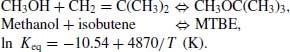
Figure 8.1 MTBE reaction system without heat integration.

The feed is composed of two streams. The first stream is a hydrocarbon stream that contains 30 mol% isobutene and 70 mol% 1-butene. The second stream, consisting of pure methanol, is in 5% molar excess of the reaction stoichiometry. The hydrocarbon feed rate is 1000 kg/h. Both streams are at 30°C and 3500 kPa. The reactor inlet temperature should be controlled at 70°C. The reactor outlet temperature will be higher than the inlet since the reaction is exothermic and a considerable amount of heat is released. This has the effect of limiting the conversion of isobutene in the reactor. The reactor product should be cooled to around 40°C so that a second reaction stage can increase the isobutene conversion to around 99%. The reactor pressure drop is 140 kPa while the pressure drops through the exchangers are 70 kPa. The exchanger volumes can be estimated at 0.1 m3 each.

Set up the temperature control loops on both heaters and coolers. Then, tune PI controllers for both of these temperature control loops. Carefully specify all the valves and pressure flow characteristics of the system. Also, you will need to add the reaction equation to the reactor and specify the equilibrium constant.

• Test your control system for disturbances in the feed rate, feed temperature and feed composition. The following disturbances are suggested as starting points for your analysis.
• Which disturbances are most difficult to control? How does the isobutene conversion vary during disturbances?
  [Hint: You may need to use a spreadsheet to calculate the isobutene conversion continuously.]

Modify the system to incorporate heat integration between the reactor outlet (hot) and the reactor feed (cold), as shown in Figure 8.2. Again, assume pressure drops of 70 kPa in both sides of the exchangers and a volume of 0.1 m3. This should also reduce the load on the existing cooler.

Figure 8.2 MTBE reaction system with heat integration.

Retune both temperature controllers. Test the new control structure against a similar range of disturbances.

• How much energy is saved by using heat integration in the process? Consider both heating and cooling duties.
• Does the system with heat integration still provide adequate control? What implications does the controllability or lack of controllability have for safety? Overall, which process configuration would you prefer?
• How could you modify the system to incorporate elements of process design to minimize utility consumption without compromising operability, controllability and safety?

Present your findings on CD, DVD or thumb drive in a short report using MS-Word. Also include on the submitted media a copy of the VMGSim files which you used to generate your findings.

References

1. Ryskamp, C.J. (1980) New strategy improves dual composition control (also effective on thermally coupled columns). Hydrocarbon Processing, June, 51–59.

2. Cutler, C.R. and Ramaker, B.L. (1979) Dynamic Matrix Control – A Computer Control Algorithm. AIChE National Meeting, Houston, 1979; Joint Auto Control Conference, San Francisco.

3. Prett, D.M. and Gillette, R.D. (1979) Optimization and Constrained Multivariable Control of a Catalytic Cracking Unit. AIChE National Meeting, Houston, 1979; Joint Auto Control Conference, San Francisco.