
Workshop 5
Controller Tuning for Capacity and Dead Time Processes
A little experience often upsets a lot of theory.
—Samuel Parks Cadman
Introduction
Prior to attempting this workshop, you should review Chapter 5 in the book.
This workshop will illustrate that VMGSim may be used to determine the appropriate parameters for a PI controller that is controlling a capacitive process with significant dead time. You will learn that controller tuning is determined by the desired load or set point response as well as the type of process and the values of the process parameters, which include process gain, time constant and dead time. A review of the two tuning techniques that are used in this workshop is provided below.
Process Reaction Curve Tuning Technique
In the process reaction curve method a process reaction curve is generated in response to a disturbance. This process curve is then used to calculate the controller gain, integral time and derivative time. The method is performed in open loop so no control action occurs and the process response can be isolated.
To generate a process reaction curve, the process is allowed to reach the steady state or as close to steady state as possible. Then, in open loop so there is no control action, a small step disturbance is introduced and the reaction of the process variable (PV) is recorded. Figure 5.1 shows a typical process reaction curve for the PV generated using the above method for a generic self-regulating process. The term self-regulating refers to a process where the controlled variable eventually returns to a stable value or levels out without external intervention.
Figure 5.1 Process reaction curve.

The process parameters that may be obtained from this process reaction curve are as follows:
Z-N Process Reaction Curve Tuning Method for a PI Controller

Auto Tune Variation (ATV) Tuning Technique
The auto tune variation or ATV technique of Åström is one of a number of techniques used to determine two important system constants called the ultimate period and the ultimate gain. Tuning values for proportional, integral and derivative controller parameters may be determined from these two constants. All methods for determining the ultimate period and ultimate gain involve disturbing the system and using the disturbance response to extract the values of these constants.
In the case of the ATV technique, a small limit cycle disturbance is set up between the manipulated variable (controller output) and the controlled variable (process variable). Figure 5.2 shows the typical ATV response plot with critical parameters defined. It is important to note that the ATV technique is applicable only to processes with dead time. The ultimate period will just equal the sampling period if the dead time is not significant.
Figure 5.2 ATV critical parameters.

General ATV Tuning Method for a PI Controller
Closed Loop Tuning Technique
The closed loop technique originally developed by Ziegler–Nichols (Z-N) is another technique that is commonly used to determine the two important system constants, ultimate period and ultimate gain. Historically speaking it was one of the first tuning techniques to be widely adopted, although it is aggressive for process control and other tuning recommendations are recommended (e.g. Cohen–Coon or IMC tuning).
In closed loop tuning, as for the ATV technique, tuning values for proportional, integral and derivative controller parameters may be determined from the ultimate period and ultimate gain. However, closed loop tuning is done by disturbing the closed loop system and using the disturbance response to extract the values of these constants.
Closed Loop Tuning Method for a PI Controller
Key Learning Objectives
Tasks
1. Tuning Controllers
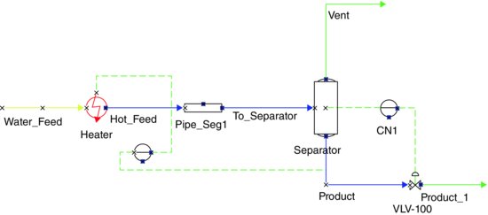
The process used for this workshop is shown in Figure 5.3. A 50/50 feed mixture of water and methanol (T = 30°C, P = 200 kPa, F = 100 kmol/h) is heated in a steam heater to approximately 70°C. The hot stream passes through a dead time lag before being stored in a separator for future use. Use a pipe segment unit operation to simulate the dead time with volume of 0.3 m3 and length of 2 m. This was the process you worked on in Workshop 4.
Figure 5.3 Illustrative capacity plus dead time process.
Set the separator level to 50% with no incoming disturbances. With the temperature controller in manual, adjust the steam valve to get a separator temperature of approximately 70°C. Bring up the temperature controller faceplate.
First use the process reaction curve technique to determine the controller settings at 50% tank level. Determine the controller settings at two more tank levels (5% and 95%).
Second, use the ATV technique to determine the controller settings.
Bring the process to a limit cycle by alternating the OP of the controller by 10% in each direction, with a constant interval between changes long enough for the PV to change by 5°C (see Figure 5.4).
- Determine the period of this limit cycle in minutes. Use this limit cycle to determine the amplitude of the temperature cycle of the stream exiting the separator and make this dimensionless by dividing by the temperature transmitter span.
- Now determine the fractional amplitude of the controller output (h).
- Calculate the ultimate gain and use this with the ultimate period to compute the controller settings.
- Determine the controller settings at two more separator levels (5% and 95%).
- Now use the closed loop tuning technique to determine the controller settings.
- Compare the results using both the ATV and Z-N tuning.
Figure 5.4 Process limit cycle.

2. Controller Contributions to Attenuation
We have seen in Workshop 3 that the process itself is able to attenuate with no control, that is, open loop. We have just tuned our feedback controller for various levels of capacitance and can now determine what the process plus control (closed loop) is able to attenuate. By subtracting the open loop attenuation from the total (closed loop) attenuation we can determine what the controller itself contributes to the overall process attenuation. Delete the pipe segment and configure the temperature controller set point to 60°C to avoid liquid feed boiling.
- Determine the total closed loop attenuation of the separator operating at the 50% level for sinusoidal disturbances of periods 10, 20, 30, 40 and 100 minutes and an amplitude of 25°C.
- Compute the controller contribution to attenuation for these disturbances.
- At 5% level determine the controller attenuation for sinusoidal disturbances of periods 5, 10, 20, 30 and 50 minutes and amplitude 25°C.
- At 95% level determine the controller attenuation for sinusoidal disturbances of periods 10, 20, 30, 40 and 100 minutes and amplitude 25°C.
- Plot attenuation versus the logarithm of the disturbance period. Briefly comment on your results.
- Dead time in the system might have a considerable negative impact on the system. Add the pipe segment back to simulate the dead time and redo all the tests above. Briefly comments on your results and findings.
Present your findings on CD, DVD or thumb drive in a short report using MS-Word. Also include on the submitted media a copy of the VMGSim files which you used to generate your findings.