5

Tuning Feedback Controllers

There is no absolute right way or, for that matter, absolute wrong way to tune a controller. Controller settings depend on what the engineer/operator deems to be good performance in terms of the desired response to process upsets. The type of process, the process gain, the time constant and dead time all play a role in determining the controller settings.

The settings also depend on the anticipated type of disturbances that the process will encounter. A controller would be tuned differently for stability due to set point changes (servo control) than for load disturbances (regulatory control). In process control systems load disturbances are most frequently encountered and, hence, most systems are optimized for regulatory control.

This chapter will discuss control quality and optimization, including the performance criteria that need to be considered when tuning a controller. A number of methods that can be used to determine controller settings in order to achieve the desired control are also described.

5.1 Quality of Control and Optimization

Controller tuning can be defined as an optimization process that involves a performance criterion related to the form of controller response and to the error between the process variable and the set point. When tuning a controller some of the questions that may be asked include

• Can offset be tolerated?
• Is no overshoot desired?
• Is a certain decay ratio required?
• Is a fast rise time needed?

These questions address some of the performance criteria that are used in the tuning of a controller, including overshoot, decay ratio and error performance.

5.1.1 Controller Response

Depending on the process to be controlled, the first consideration is to decide what type of response is optimal, or at least acceptable. Typical process responses to a load change are illustrated in Figure 5.1.

Figure 5.1 Typical responses to a load change.

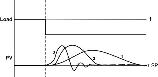
The three possible general extremes of response that exist, as shown in Figure 5.1, are

From these three general extremes, we can see that the selection of good control is a tradeoff between the speed of response and deviation from the set point. A highly tuned controller may become unstable if large disturbances occur, whereas a sluggishly tuned controller provides poor performance but is very robust. What is typically required for most process control loops is a compromise between performance and robustness.

When examining the response, there are several common performance criteria that can be used for controller tuning, which are based on the characteristics of the system's closed loop response. Some of the more common criteria include overshoot, offset, rise time and decay ratio. Of these simple performance criteria, control practitioners most often use decay ratio.

Cyclic Radian Frequency

The cyclic radian frequency, ω, is defined as

(5.1)

and

(5.2)

If Equation 5.2 is substituted into Equation 5.1, we obtain

(5.3)

The cyclic radian frequency can also be related to the undamped natural frequency, ωn, and the damping coefficient, ξ:

(5.4)

Overshoot

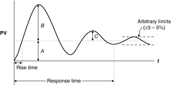
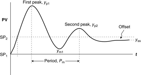
Overshoot is the amount the response exceeds the steady-state final value. Referring to Figure 5.2, the overshoot can be defined as

(5.5)

Figure 5.2 Second- or higher-order typical response to a set point change.

Decay Ratio

The decay ratio is the ratio of the amplitude of an oscillation to the amplitude of the proceeding oscillation, C/B in Figure 5.2. More specifically, we can define the quarter decay ratio (QDR), which lies between critical damping and underdamping:

(5.6)

The decay ratio is often used to establish whether the controller as tuned is providing a satisfactory response. The QDR or similar has been shown through experience to provide a reasonable tradeoff between minimum deviation from the set point after an upset and the fastest return to the set point. The penalty of QDR is that some oscillation does occur, leading to many recommending less than QDR for process control. For a second-order system it can be shown that

(5.7)

Rise Time

The rise time is the time required by the transient response to initially reach the final steady-state value.

Response Time

The response time is the time required for the response to settle within the specified arbitrary limits. These limits are typically set at ± 3–5% of the PV steady-state value.

5.1.2 Error Performance Criteria

The previously discussed simple performance criteria, that is, decay ratio, overshoot, and so on, use only a few points in the response and therefore are simple to use. On the other hand, error performance criteria are based on the entire response of the process but they are also more complicated.

Integrated Error

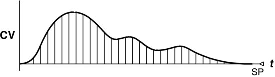
The curve shown in Figure 5.3 represents the response of a loop due to a process upset. This graphical representation of the controlled variable's return to the set point is known as a response curve. The integrated error (IE) is the area under the response curve, and the idea of using this as an error criterion is to attempt to minimize this area.

Figure 5.3 General response curve.

In mathematical terms, with e representing the error as a function of time, we can write

(5.8)

It may not always be possible to minimize IE without paying a penalty in some respect. For example, underdamping produces a minimum area under the response curve but has considerable oscillation.

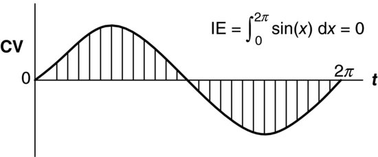
The method of IE may not be 100% reliable if there is no averaging elsewhere in the process. For example, if there is a sinusoidal oscillation about the set point, the positive and negative areas tend to cancel each other out over time, which presents a misleading conclusion, as shown in Figure 5.4. However, barring this situation, IE is a perfectly adequate error criterion.

Figure 5.4 Sinusoidal error response.

Integrated Absolute Error

Integrated absolute error (IAE) essentially takes the absolute value of the error. Negative areas are accounted for when IAE is used, thus dismissing the problem encountered with IE regarding sinusoidal responses:

(5.9)

Integrated Squared Error

The integrated squared error (ISE) criterion uses the square of the error, thereby penalizing larger errors more than smaller errors. This gives a more conservative response, that is, faster return to the set point:

(5.10)

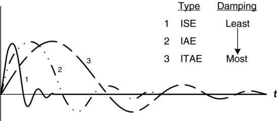
Integrated Time Absolute Error

The integrated time absolute error (ITAE) criterion is the integral of the absolute value of the error multiplied by time. ITAE results in errors existing over time being penalized even though they may be small, which results in a more heavily damped response:

(5.11)

Figure 5.5 shows the various responses of a loop that is tuned to the above criteria, including IAE, ISE and ITAE.

Figure 5.5 Response to various error criteria.

5.2 Tuning Methods

The following presents a very brief description of some of the various accepted methods used for controller tuning. In each case the suggested controller settings are optimized for a particular error performance criterion, often QDR. The first method described is based entirely on trial and error, while the rest are based upon some understanding of the physical nature of the process to be controlled. This understanding is generated from either open or closed loop process testing.

5.2.1 ‘Trial and Error’ Method

As the name suggests, tuning by trial and error is simply a guess and check type method. The following is a list of practical suggestions for tuning a controller by trial and error. These suggestions are also useful for retuning or fine-tuning controllers tuned by other methods:

Rules of Thumb

The following rules of thumb should not be taken as gospel or as a methodology but rather are intended to indicate typical values encountered. As such, these rules can be useful when tuning a controller using the trial and error method. However, it is important to remember that controller parameters are strongly dependent upon the individual process and may not always abide by the rules outlined below.

Flow

When dealing with a flow loop, P-only control can be used with a low controller gain. For accuracy, PI control is used with a low controller gain and high integral action. Derivative action is not used because flow loops typically have very fast dynamics and flow measurement is inherently noisy:

Level

Levels represent material inventory that can be used as surge capacity to dampen disturbances. Hence, loosely tuned P-only control is sometimes used. However, most operators do not like offset, so PI level controllers are typically used.

The following P-only settings ensure that the control valve will be 50% open when the level is at 50%, wide open when the level is at 75% and shut when the level is at 25%:

Typical PI controller settings are

Pressure

Pressure control loops show large variation in tuning depending on the dynamics of the pressure response. Typical ranges are as follows:

Temperature

Temperature dynamic responses are usually fairly slow, so PID control is used. Typical parameter values are

5.2.2 Process Reaction Curve Methods

In the process reaction curve methods a process reaction curve is generated in response to a disturbance. This process curve is then used to calculate the controller gain, integral time and derivative time. These methods are performed in open loop so no control action occurs and the process response can be isolated.

To generate a process reaction curve, the process is allowed to reach steady state or as close to steady state as possible. Then, in open loop so there is no control action, a small disturbance is introduced and the reaction of the process variable is recorded. Figure 5.6 shows a typical process reaction curve generated using the above method for a generic self-regulating process. The term self-regulating refers to a process where the controlled variable eventually returns to a stable value or levels out without external intervention.

Figure 5.6 Process reaction curve.

The process parameters that may be obtained from this process reaction curve are as follows:

L is the lag time (min); T is the time constant estimate (min); P is the initial step disturbance (%); ΔCp is the change in PV in response to step disturbance, (change in PV)/(PV span) × 100, (%); is the reaction rate (%/min); and is the lag ratio (dimensionless).

Methods of process analysis with forcing functions other than a step input are possible and include pulses, ramps and sinusoids. However, step function analysis is the most common as it is the easiest to implement.

Ziegler–Nichols Open Loop Rules

In 1942, Ziegler and Nichols [1] changed controller tuning from an art to a science by developing their open loop step function analysis technique, which is the basis of the general process reaction curve technique. They also developed a closed loop technique, which is described in the next section on constant cycling methods.

The Ziegler–Nichols open loop-recommended controller settings for QDR are as follows:

(5.12)

(5.13)

(5.14)

(5.15)

(5.16)

(5.17)

These settings should be taken as recommendations only and tested thoroughly in closed loop, fine-tuning the parameters to obtain QDR or whatever is the desired response criterion. It is worthwhile noting that for chemical process control, Ziegler–Nichols recommendations are often considered very aggressive as they were designed for servo control for US Naval applications and not process control. Consequently, tuning may have to be adjusted or fine-tuned for process control application (lower gain, higher integral time). Also, other workers have developed a series of less aggressive recommendations, often with less than QDR as a desirable response criterion.

Cohen–Coon Open Loop Rules

In 1953, Cohen and Coon [2] developed a set of controller tuning recommendations that correct for one deficiency in the Ziegler–Nichols open loop rules. This deficiency is the sluggish closed loop response given by the Ziegler–Nichols rules in the relatively rare occasion when process dead time is large relative to the dominant open loop time constant. In other regards, the Cohen–Coon recommendations are still considered relatively aggressive for process control.

The Cohen–Coon-recommended controller settings are as follows:

(5.18)

(5.19)

(5.20)

(5.21)

(5.22)

(5.23)

As with the Ziegler–Nichols open loop method recommendations, the Cohen–Coon values should be implemented and tested in closed loop and adjusted accordingly to achieve QDR and are also usually considered aggressive so that de-tuning may be required.

Internal Model Control Tuning Rules

As mentioned above, many practitioners have found that the Ziegler–Nichols open loop and Cohen–Coon rules are too aggressive for most chemical industry applications since they give a large controller gain and short integral time. Rivera et al. [3] developed the internal model control (IMC) tuning rules with robustness in mind. The tuning parameter from the IMC method (the closed loop speed of response) relates directly to the closed loop time constant and the robustness of the control loop. As a consequence, the closed loop step load response exhibits no oscillation or overshoot. Lambda tuning, for example [4], is a term that is also used to refer to controller tuning methods that are based on a specified closed loop time constant. More recently Skogestad has proposed IMC tuning rules that have also been shown to exhibit superior performance in a number of studies [5]. Since the general IMC method is unnecessarily complicated for processes that are well approximated by first-order dead time or integrator dead-time models, simplified IMC rules were developed by Fruehauf et al. [6] for PID controller tuning (see Table 5.1).

Table 5.1 Simplified IMC rules [6].

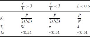
Of course, these recommendations need to be tested in the closed loop situation and the final settings arrived at through the use of fine-tuning.

5.2.3 Constant Cycling Methods

Ziegler–Nichols Closed Loop Method

The closed loop technique of Ziegler and Nichols [1] is a technique that is commonly used to determine the two important system constants, ultimate period and ultimate gain. It was one of the first tuning techniques to be widely adopted.

When tuning using Ziegler–Nichols closed loop method, values for proportional, integral and derivative controller parameters may be determined from the ultimate period and ultimate gain. These are determined by disturbing the closed loop system and using the disturbance response to extract the values of these constants.

The following is a step-by-step approach to using the Ziegler–Nichols closed loop method for controller tuning:

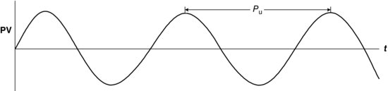
Figure 5.7 Constant amplitude limit cycle.

Yuwana–Seborg Closed Loop Tuning

Another closed loop method that retains the advantage of being performed under control in the loop but addresses the disadvantage of the oscillatory response that results from the Ziegler–Nichols technique is that of Yuwana–Seborg [7]. The technique is based on the assumption that the plant dynamics, while unknown, can be approximated by a first-order plus dead-time model of process gain, Kp, time constant, τ, and dead time, L. The method is briefly as follows:

Table 5.2 Yuwana–Seborg tuning recommendation constants.

Figure 5.8 Typical response of a stable first-order plus dead-time system using P control.

The algorithm is actually quite easy to implement. The main challenge is the reliable determination of the peaks and troughs.

Auto Tune Variation Technique

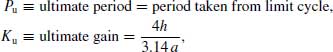
The auto tune variation (ATV) technique of Åström and Hagglund [8] is another closed loop technique used to determine the two important closed loop system constants, the ultimate period and the ultimate gain. However, the ATV technique determines these system constants without unduly upsetting the process. Tuning values for proportional, integral and derivative controller parameters can be determined from these two constants. Here we recommend the use of Tyreus–Luyben [9] settings for tuning that is suitable for chemical process unit operations. All methods for determining the ultimate period and ultimate gain involve disturbing the system and using the disturbance response to extract the values of these constants.

In the case of the ATV technique, a small limit cycle disturbance is set up between the manipulated variable (controller output) and the controlled variable (process variable). Figure 5.9 shows the instrument setup, and Figure 5.10 shows the typical ATV response plot with critical parameters defined. It is important to note that the ATV technique is applicable only to processes with significant dead time. The ultimate period will just equal the sampling period if the dead time is not significant.

Figure 5.9 ATV tuning instrument setup.

Figure 5.10 ATV critical parameters.

General ATV tuning method for a PI Controller is as follows:

(5.41)

(5.42)

Comparison of ATV and Ziegler–Nichols Closed Loop Tuning Techniques

Table 5.3 compares the tuning constants between the ATV and Ziegler–Nichols closed loop (Z-N CL) tuning techniques. Notice that the Ziegler–Nichols tuning is more aggressive with a larger controller gain and shorter integral time. This technique was originally developed for electromechanical systems control and is based on the more aggressive QDR criterion. ATV tuning was developed for fluid and thermal processes and emphasizes minimizing overshoot. ATV is, therefore, often the preferred technique for process control.

Table 5.3 Tuning comparison.

References

1. Ziegler, J.G. and Nichols, N.B. (1942) Optimum settings for automatic controllers. Transactions of the ASME, 64, 759.

2. Cohen, G.H. and Coon, G.A. (1953) Theoretical consideration of retarded control. Transactions of the ASME, 75, 827.

3. Rivera, D.E., Morari, M. and Skogestad, S. (1986) Internal model control, 4. PID controller design. Industrial and Engineering Chemistry Process Design and Development, 25, 252.

4. McMillan, G.K. (ed.) (1999) Process/Industrial Instruments and Controls Handbook, 5th edn, McGraw-Hill, New York, NY.

5. Skogestad, S. (2003) Simple analytic rules for model reduction and PID controller tuning, Journal of Process Control, 13(4), 291–309.

6. Fruehauf, P.S., Chien, I.-L. and Lauritsen, M.D. (1993) Simplified IMC-PID tuning rules. ISA, Paper# 93-414, p. 1745.

7. Yuwana, M. and Seborg, D.E. (1982) A new method for on-line controller tuning. AIChE Journal, 28, 434.

8. Åström, K.J. and Hagglund, T. (1984) Automatic tuning of simple regulators with specifications on phase and amplified margins. Automatica, 20, 645.

9. Tyreus, B.D. and Luyben, W.L. (1992) Tuning of PI controllers for integrator/deadtime processes. Industrial and Engineering Chemistry Research, 31, 2625.