
2
Process Control Hardware Fundamentals
In order to analyse a control system, the individual components that make up the system must be understood. Only with this understanding can the workings of a control system be fully comprehended. The rest of this book deals extensively with controller and process characteristics. It is therefore appropriate and necessary that hardware fundamentals for the primary elements and final control elements be studied first in this chapter. Discussion of controller hardware is delayed until Chapter 4, where the control equations governing the controllers are covered. Several of the concepts introduced in this chapter are discussed in further detail in later sections of this book.
2.1 Control System Components
A control system is comprised of the following components:
Figure 2.1 illustrates a level control system and its components. The level in the tank is read by a level sensor device, which transmits the information on to the controller. The controller compares the level reading with the desired level or set point and then computes a corrective action. The controller output adjusts the control valve, referred to as the final control element. The valve percent opening has been adjusted to correct for any deviations from the set point.
Figure 2.1 Surge tank level controller.

Figure 2.2 is an information flow diagram that corresponds to the physical process flow diagram in Figure 2.1. The information is transmitted between the different control system elements as either pneumatic, electronic or digital signals. These signals often use a live zero. Typical levels are 20–100 kPa (or 3–15 psi) for pneumatic signals, a 4–20 mA current loop that is often converted to 1–5 V for analog electronic signals and binary digits or bits for digital signals.
Figure 2.2 Single-input/single-output block diagram.

2.2 Primary Elements
Primary elements, also known as sensors/transmitters, are the instruments used to measure variables in a process such as temperature and pressure. A full listing of the types of primary elements available on the market would be very long, but these sensor types can be broadly classified into groups including the following:
Some specific examples of instruments from the more common groups listed above will be examined, including pressure, level, temperature and flow. It is important to note that this list is not complete or fully representative of the complex developments in this area. This later point applies particularly to quality or analysis instruments which are only briefly introduced here. Further information and detail can be found in the references.
2.2.1 Pressure Measurement
There are numerous types of primary elements used for measuring pressure that could be studied; however, this discussion will be limited to some of the most common types encountered. These include manometers, Bourdon tubes and differential pressure (DP) cells.
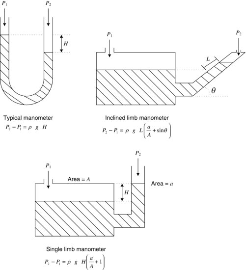
Manometers
Manometers are simple, rugged and cheap and give reliable static measurements. They are, therefore, very popular as calibration devices for pressure measurement. The working concept of a manometer is simple. A fluid with a known density, ρ, is used to measure the pressure difference between two points, P1–P2, based on Equation 2.1, where H is the height difference in the fluid level:
Figure 2.3 illustrates some of the different manometer types.
Figure 2.3 Various manometer types.
The Bourdon Tube Pressure Gauge
The Bourdon tube pressure gauge, named after Eugene Bourdon (ca. 1852) and shown in Figure 2.4, is probably the most common gauge used in industry. Figure 2.4 illustrates the Bourdon tube pressure gauge. The essential feature of the Bourdon tube is its oval-shaped cross section. The operating principle behind the gauge is that when pressure is applied to the inside of the tube the tip is moved outward. This pulls up the link and causes the quadrant to move the pinion to which the pointer is attached. The resultant movement is indicated on a dial. A hairspring is also included (not shown) to take up any backlash that exists between quadrant and pinion; this has no effect on calibration.
Figure 2.4 Bourdon tube pressure gauge.

The accuracy of the gauge is ±0.5% of full range for commercial models. Generally, the normal working pressure will be specified as 60% of the full scale.
Other types of these gauges include the twist tube, spiral tube and helical tube. Diaphragm and bellows gauges are two other types of pressure sensors that were developed later. For more details on Bourdon tube materials and design refer to Giacobbe and Bounds [1], Goitein [2] and Considine [3].
The Differential Pressure Cell
The DP cell is considered by many as the start of modern-day automation. The DP cell was developed at the outbreak of World War II by Foxboro in Massachusetts, USA, on a government grant provided that it was not patented. The idea was that competition would bring down the price of the instrument.
DP cells allow remote transmission to central control rooms where a small number of operators can control large, complex plants. For example, a typical petroleum refinery processing around 80 000 barrels/day (530 m3/h) might have 2000 DP cells throughout the refinery.
Seal systems can be used to enhance the usefulness of the DP cell by facilitating pressure measurement for many temperature ranges (−73–427°C) [4]. They serve to protect the transmitter from the process fluid, using a hydraulic system to conduct the pressure from the process fluid to the transmitter. Only the seal's diaphragm contacts the process fluid, and a capillary or tube of fluid transfers the process pressure from the diaphragm to the transmitter. Before a seal is installed consider ambient conditions, such as temperature, which may introduce errors.
Some of the major benefits of DP cells are that their maintenance is practically zero and no mercury is used in the operation of the transducer.
The Pneumatic DP Cell
Figure 2.5 shows a schematic of a pneumatic DP cell.
Figure 2.5 Pneumatic DP cell (Reproduced by permission of Emerson Process Management).
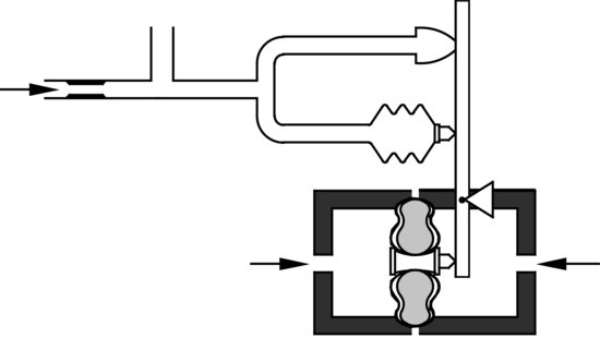
Pressure is applied to the opposite sides of a silicone-filled twin diaphragm capsule. The pressure difference applies a force at the lower end of the force bar, which is balanced through a simple lever system consisting of the force bar and baffle. This force exerted by the capsule is opposed through the lever system by the feedback bellows. The result is a 3 psi (or 20 kPa if calibrated in SI units) to 15 psi (or 100 kPa if calibrated in SI units) signal proportional to the DP. The range of the cell is 1.20–210 kPa DP with an accuracy of ±0.5% of the range.
Modern DP Cells
E-type electronic transducers, strain gauges, capacitive cell transducers and most recently digital electronics have replaced the pneumatic-type DP cell. Figure 2.6 shows a schematic of an electronic DP cell. Figure 2.7 is a photo of a modern DP cell.
Figure 2.6 Electronic DP cell (Reproduced by permission of Emerson Process Management).
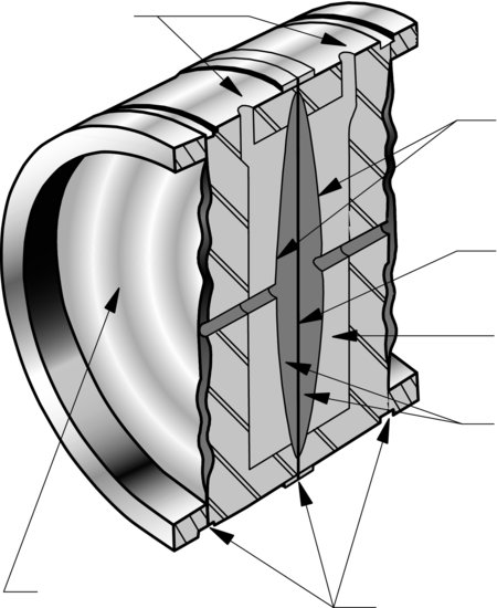
Figure 2.7 Model 3051 electronic DP cell (Reproduced by permission of Emerson Process Management).
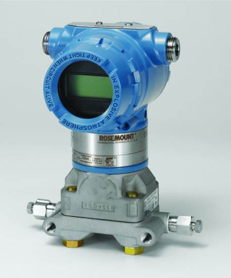
The features of the modern electronic DP cell, such as the Rosemount Model 3051 or Honeywell's ‘smart’ transmitter [5], include remote range change, diagnostics that indicate the location and type of any system faults, easy self-calibration, local digital display, reporting and interrogation functions and local and remote reporting. The modern DP cell can also be directly connected to a process computer and has the ability to communicate with the computer indicating problem analysis that is then displayed on the computer screen.
2.2.2 Level Measurement
Level measurement is the determination of the location of the interface between two fluids which separate by gravity, with respect to a fixed plane. The most common level measurement is between a liquid and a gas. Methods of level measurement include the following [6,7]:
It is extremely important that vessels are well protected from an overflow condition. An overflowing vessel may have severe safety consequences, impacting nearby employees, the environment and the surrounding community. Some vessels require low-level protection to operate safely. Ideally, each vessel should have a visual indication for the operator, an alarm point and a transmitted level indicator [8].
Factors affecting the choice of level measurement include corrosive process fluids (requiring exotic materials), viscous process fluids which may cause blockages, hazardous atmospheres, sanitary requirements, density changes, dielectric and moisture changes and the required degree of accuracy and durability.
Pressure/head devices such as the DP cell are the most popular of all level measurements devices. The DP cell can often be used where manometers are impracticable and floats would cause problems. The DP cell requires a constant product density for accurate measurement of level or a way of compensating for density fluctuations. Figure 2.8 demonstrates a typical set-up for level measurement using a Rosemount Model 3051SMV level controller, which is essentially a combined DP cell and proportional controller.
Figure 2.8 Model 3051SMV multivariable level controller in a liquid level process (Reproduced by permission of Emerson Process Management).

Ultrasonic Methods
Ultrasonic refers to sound of such high frequency that it is undetectable to the human ear. Frequencies used in level measurement range from 30 kHz to the megahertz range [9].
A transducer sends pulses of ultrasonic sound to the surface of the liquid to be measured. The liquid surface reflects these pulses and the distance from transducer to the liquid level is calculated. This calculation is based on the speed of the signal and the time elapsed between the sending and receiving of the ultrasonic sound signal (Figure 2.9).
Figure 2.9 Ultrasonic level transmitter (Reproduced from [9]).
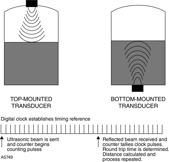
Ultrasonics can be top or bottom mounted. Although a top-mounted device is easier to service, mists, vapours and internal ladders and agitators may cause erroneous readings. Bottom-mounted devices must be calibrated to the density of the measured fluid; however, bubbles and solids in the liquid may skew their reading [9].
2.2.3 Temperature Measurement
Methods of measuring temperature include [5]
Bimetal thermostats, thermocouples and resistance thermometers will be discussed in detail.
Bimetal Thermostats
The bimetal thermostat works on the concept that different metals expand by different amounts if they are subject to the same temperature rise. If two metals are fixed rigidly together, then a differential expansion takes place when the metals are heated, causing the composite bar to bend. The thermostat employs the bimetal bar to switch on or off a control device depending on the temperature. An illustration of a bimetal thermostat is given in Figure 2.10.
Figure 2.10 Bimetal thermostat.
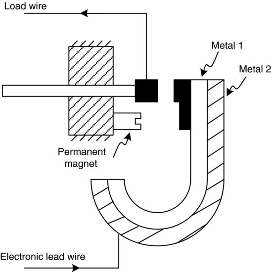
The temperature range for bimetal thermostats is 0–400°C with an accuracy of ±5%, although the accuracy can be increased to ±1% [6]. The deflection/temperature relationship is linear for many metal combinations over a particular temperature range only, and the materials must be chosen with care. These instruments are rugged and cheap, offer direct reading and can work under conditions of vibration.
Thermocouples
When two dissimilar metal or alloy wires are joined together at both ends to form a loop and a difference in temperature exists between the ends, a difference in junction potentials exists resulting in a thermoelectric electromagnetic field (emf). This is known as the Seebeck effect, after Seebeck's 1821 discovery of this phenomenon. The magnitude of the emf will depend on the types of materials used and the temperature difference. This is the concept behind a thermocouple for measuring temperature.
If one junction temperature, the reference or cold junction, is maintained at a constant and known value and the characteristics of the thermocouple are known, then the magnitude of the emf generated will be a measure of the temperature of the other junction. This other junction is called the hot junction.
The emf generated for any two particular metals at a given temperature will be the same regardless of the size of the wires, the areas in contact or the method of joining them together. The relationship between temperature and generated emf is non-linear except over limited ranges. On the steep part of the curve, the relationship is
In Equation 2.2, e is the generated emf, T1 and T2 are the hot and cold junction temperatures in Kelvin and a and b are constants for the given material. An example of the relation is given in Figure 2.11 for a Cu/Fe thermocouple system.
Figure 2.11 Relationship between temperature and emf for a Cu/Fe system.

Thermocouple Types
There are many thermocouple types. Common systems and their ranges are as follows:
Base metal thermocouple types:
Noble metal thermocouple types:
Poisons to Thermocouples
- Iron (Fe) deteriorates quickly due to scaling in oxidizing atmospheres at high temperatures.
- Chromel and alumel thermocouples are poisoned by gases that are carbon based, are sulphurous, or contain cyanide groups. These thermocouples are better in an oxidizing atmosphere than a reducing atmosphere.
- Platinum must be protected from hydrogen and metallic vapours.
Resistance Thermometer Detectors (RTDs)
RTDs are made of either metal or semiconductor materials as resistive elements that may be classed as follows [3]:
An example is the platinum RTD, which is the most accurate thermometer in the world.
RTDs exhibit a highly linear and stable resistance versus temperature relationship. However, resistance thermometers all suffer from a self-heating effect that must be allowed for, and I2R must be kept below 20 mW, where I is defined as the electrical current and R is the resistance.
When compared to thermocouples, RTDs have higher accuracy, better linearity and long-term stability, do not require cold junction compensation or extension lead wires and are less susceptible to noise. However, they have a lower maximum temperature limit and are slower in response time in applications without a thermal well (a protective well filled with conductive material in which the sensor is placed).
Selecting Temperature Sensors
Getting the right operating data is crucial in selecting the proper sensor. A good article on selecting the right sensor is by Johnson [10].
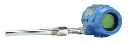
Figure 2.12 shows a selection of thermocouples, RTDs and temperature accessories, such as thermal wells, that are typically available from instrument suppliers (in this case Emerson Process Management). Figure 2.13 shows a picture of a typical temperature sensor and transmitter assembly.
Figure 2.12 Selection of thermocouples, RTDs and accessories (Reproduced by permission of Emerson Process Management).
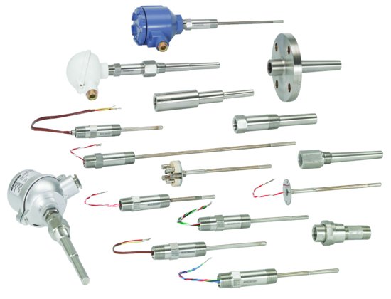
Figure 2.13 Temperature sensor and transmitter assembly (Reproduced by permission of Emerson Process Management).
2.2.4 Flow Measurement
Flow measurement techniques can be divided into the following categories [3]:
Selection of a flowmeter is based on obtaining the optimum measuring accuracy at the minimum price. It should be noted that flowmeters may use up a substantial amount of energy, especially when used in low pressure vapour service. Therefore they should only be provided when necessary [8].
There are many factors to consider when selecting a flowmeter, including properties of the fluid being measured such as viscosity, and performance requirements such as response time and accuracy. Ambient temperature effects, vibration effects and ease of maintenance should also be compared when selecting a flowmeter. For a more thorough presentation on the selection of flowmeters, refer to the article by Parker [11].
Orifice plates and magnetic flowmeters will be discussed in detail since they are two of the most common types found in the fluid-processing industry.
Orifice Plates
The concentric orifice plate is the least expensive and the simplest of the head meters. The orifice plate is a primary device that constricts the flow of a fluid to produce a DP across the plate. The result is proportional to the square of the flow. Figure 2.14 shows a typical thin-plate orifice meter.
Figure 2.14 Thin-plate orifice meter.
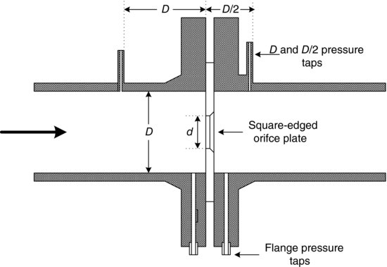
An orifice plate usually produces a larger overall pressure loss than other primary devices. A practical advantage of the orifice plate is that cost does not increase significantly with pipe size. They are used widely in industrial applications where line pressure losses and pumping costs are not critical.
The thin concentric orifice plate can be used with clean homogenous fluids, which include liquids, vapours or gases, whose viscosity does not exceed 65 cP at 15°C. In general the Reynolds number (Re) should not exceed 10 000. The plate thickness should be 1.5–3.0 mm or, in certain applications, up to 4.5 mm [12].
Many variations for orifice plates have been suggested, especially during the 1950s when oil companies and universities in North America and Europe sponsored numerous PhD studies on orifice plates [3]. Of these only a few have survived, which were the ones that incorporated cheaply some of the features of the more expensive devices. Figure 2.15 shows some of these designs. Other designs that are utilized include eccentric and segmental orifice configurations.
Figure 2.15 Various orifice plate designs.

Magnetic Flowmeters
The magnetic flowmeter is a device that measures flow using a magnetic field, as implied by the name. The working relationship for magnetic flowmeters is based on Faraday's law (see Equation 2.3), which states that a voltage will be induced in a conductor moving through a magnetic field:
In Equation 2.3, E is the generated emf, B is the magnetic field strength, D is the pipe diameter, V is the average velocity of the fluid and k is a constant of proportionality. As seen in Equation 2.3, when k, B and D are kept constant, V is proportional to E.
Figure 2.16 illustrates the principle of operation of a magnetic flowmeter. In the past, magnetic flowmeters have been very expensive compared to orifice plates and DP cells. However, now the cost is very competitive, and in fact magnetic flowmeters are replacing orifice plates where possible.
Figure 2.16 Views of the Model 8705 magnetic flowmeter with junction box (Reproduced by permission of Emerson Process Management).

There are numerous benefits to using a magnetic flowmeter. With polytetrafluoroethylene (PTFE), fibreglass or rubber liners, the magnetic flowmeter can handle almost any corrosive liquid. The electrodes can be made from very corrosive-resistant metals. Gold, titanium and tantalum have been used in the past. The magnetic flowmeters are virtually maintenance free, and there is no flow obstruction to the stream being measured. Also, they can be readily connected to an electronic controller and can give out a digital signal that can be directly fed to a computer.
When using a magnetic flowmeter it is necessary that the liquid be conductive, although low conductivities are acceptable. Also, outside capacitance can create a big problem. Calibration should be done carefully initially, with accurate readings done on the liquid conductivity to ensure accurate set-up of the magnetic flowmeter. Note too that proper grounding is critical to magmeter performance to ensure the magnetic field remains isolated from magnetic noise of nearby electrical equipment.
Vortex meters (Figure 2.17) utilize the von Kármán effect. This effect is readily observable when the wind blows and a flag flaps in the wind. In a vortex meter, fluid alternately separates from each side of the shedder bar face. Vortices form behind the face and cause alternating DPs around the back of the shedder bar. The frequency of the alternating vortex development is linearly proportional to the flow rate. The flexing motion is sensed by a piezoelectric sensor element which converts the motion to an alternating electric signal. Vortex flowmeters are suitable for liquids, gas and steam. They are the most cost effective in smaller lines (6 in. and smaller). It is important to recognize that this meter type has a low flow cut-off and does not measure to zero.
Figure 2.17 Model 8800 vortex flowmeter (Reproduced by permission of Emerson Process Management).

Coriolis flowmeters (Figure 2.18) make use of the Coriolis effect. The inertia force must be taken into consideration if Newton's law of motion of bodies is to be used in a rotating frame of reference. As the flow passes through, the Coriolis meter tubes twist a bit. The amount of deflection is measured and used to determine the flow rate, but can also be used to determine temperature and density. This flow device is mechanically tolerant, can measure two-phase flow, does not require flow conditioning or straight pipe run lengths and is low maintenance.
Figure 2.18 Coriolis flowmeter (Reproduced by permission of Emerson Process Management).

A summary of the strengths and weaknesses of different flowmeters in various applications is highlighted in Figure 2.19.
Figure 2.19 Coriolis flowmeter (Reproduced by permission of Spartan Controls Ltd).

2.2.5 Quality Measurement and Analytical Instrumentation
Primary elements include the rapidly growing range of analytical instrumentation. Chemical engineering graduates need at least an awareness of what is now measurable. For example flue gas oxygen (and CO) analysers are commonplace. Gas and liquid densitometers are used extensively in industry. Other common analysers include viscometers, calorimeters and chromatographs. Near infrared (NIR) spectroscopy has become very widely used as a general-purpose inferential composition measurement technique and nuclear magnetic resonance (NMR) spectroscopy looks like it could go the same way in a decade or so. The oil industry is also a big user of analysers for vapour pressure, flash point, distillation and cloud point. However, because of the specialized and detailed nature of these instruments, which are more the domain of physical chemistry, the reader is referred to the Process Industrial Instruments and Controls Handbooks by Considine [3] and McMillan and Considine [13] and the specialist book Process Analyzer Technology by Clevett [14] for further details.
2.2.6 Application Range and Accuracy of Different Sensors
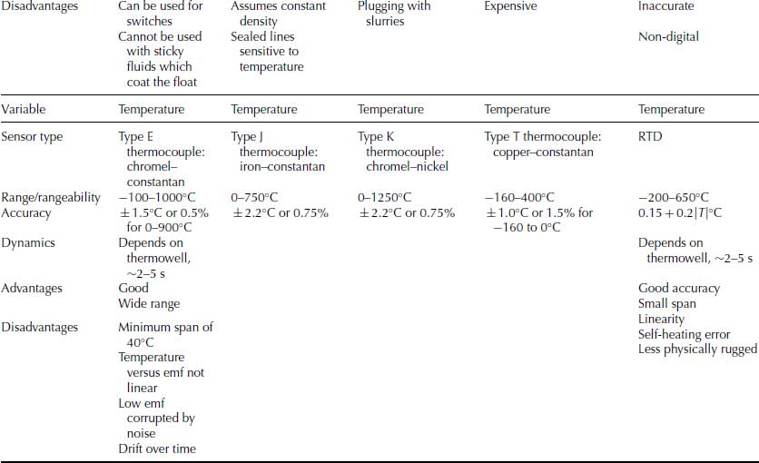
Table 2.1 shows the application range and accuracy of most of the different sensors mentioned in the foregoing subsections. More details can be obtained from the books by Considine [3], McMillan and Considine [13] and Clevett [14], and of course instrumentation vendors.
Table 2.1 Application range and accuracy of sensors (Adapted from Marlin [15]).

2.3 Final Control Elements
Pneumatic, or air-operated, diaphragm control valves are the most common final control element in process control applications. They are used to regulate the flow of material or energy into a system. Variable speed pumps are also possible but are often costly as motor control is expensive, are less efficient, break down more often and maintain maximum pressure if they fail. Electric valves are seen, but only for large applications above 25 cm pipe/valve diameters. Variable electric power control elements such as rheostats are used in small applications such as laboratory water bath temperature control.
Since control valves are the most common final control element we will now devote our discussion to control valves.
2.3.1 Control Valves
Since process engineers tend to dedicate their time to tuning control loops, the significance of the performance of the control valve is often overlooked. ‘As much as 80% of all process variability can be attributed to poor control valve performance (i e. how quickly and accurately the control valve responds to the control signal)’ [16].
The components that control a valve are [16]
The control valve components are illustrated with a butterfly valve in Figure 2.20.
Figure 2.20 Control valve cutaway (Reproduced by permission of Emerson Process Management).
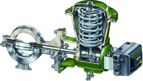
The sliding stem control valves are the most common control valve configuration and have at least half the market in control valves. Figures 2.21a and b show a typical, modern sliding stem control valve assembly.
Figure 2.21 (a) Typical modern sliding stem control valve assembly; (b) single-acting spring return actuator and digital valve positioner for a modern sliding stem control valve (Reproduced by permission of Emerson Process Management).

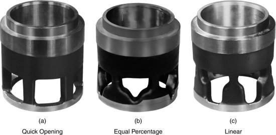
The pneumatic diaphragm-operated control valve is the most commonly specified final control element in existence. Pneumatic valves have many advantages over electrically activated valves, but the main ones are initial lower purchase cost, relative ease of maintenance, speed of response and developed power of the valve plug. This last reason has become less relevant in recent times since the valve bodies have changed from contoured and ported styles to plug and cage styles in order to avoid unbalanced forces in single ported designs, especially for high-pressure liquids. Figure 2.22 shows some of the newer styles of valve cages.
Figure 2.22 Characterized cages for globe-style valve bodies (Reproduced by permission of Emerson Process Management).
Control Valve Sizing
The common equation for the flow of a non-compressible fluid through a control valve is given in Equation 2.4 [17], which can be derived from Bernoulli's equation:
In Equation 2.4, Q is the volumetric flow rate and ΔP is the pressure drop across the valve, SG is the relative density compared to water, and Cv is the valve coefficient. Cv is defined by convention in field or imperial units as the number of US gallons that will pass through a control valve in 1 minute, when the pressure differential across the valve is 1 psi.
Cv varies negligibly with Re for most valve applications. Even in cases where the Reynolds number is low, the Reynolds number at the valve will be high due to the valve restricting flow, and so the valve is normally operating in a region where Cv is independent of the Reynolds number. For valves with a streamlined shape such as those used for slurries or very viscous liquids, the Reynolds number can be low enough that Cv becomes dependent. In these cases a correction factor for the low Cv is usually supplied in the manufacturers' catalogues under the heading ‘Viscosity Correction Factors for Cv’ [17–21].
The value of Cv is also a function of A, which is the flow area of the valve. For a given valve, this value of A varies extensively with valve opening. The curve giving the variation of Cv at high Reynolds number with valve opening is called the ‘inherent characteristic of the valve’. The maximum value of Cv occurs when the valve is wide open and depends on the design and size of the valve. For geometrically similar valves, Cv is proportional to the valve size.
Inherent Valve Characteristic
The inherent characteristic of a valve is a plot of Cv versus valve opening. This curve is usually plotted as Cv in % of maximum flow (or Cv). Inherent characteristics are usually plotted in this way rather than actual Cv versus actual lift so that the same curve will apply to a set of geometrically similar valves, irrespective of size. If the characteristic curve and the maximum Cv are known then the Cv at any intermediate lift or opening can be determined.
Three common examples of operating valve characteristics are quick opening, linear and equal percentage, as illustrated in Figure 2.23.
Operating Characteristic
The operating characteristic is a plot of flow versus lift, where lift refers to valve opening, for a particular installation. This is not an inherent property of the valve and is usually plotted as flow versus lift in a similar way to the inherent characteristic, with both the flow and the lift being plotted as a percentage of the maximum.
If the pressure drop did not change across the valve with valve opening, then the flow would vary proportionally with Cv, and thus the operating characteristic would be the same as the inherent characteristic curve if both were plotted as percentage of maximum. However, as the valve closes, the pressure drop across it increases. This increased ΔP is due to the fact that as the valve resistance increases, the valve's resistance becomes a larger fraction of the total system resistance. This is because as the valve closes, flow through the system decreases and the system ΔP other than the valve decreases but the valve ΔP increases. This means that as the valve closes, its Cv falls but its ΔP increases. The result is that the flow does not fall as fast as the Cv, and so the installed or operating flow characteristic differs from the inherent characteristic.
When the valve is shut its resistance is infinite and the whole available pressure drop occurs across it. Thus the ΔP across the valve varies from a maximum when closed, to a minimum when 100% open. The greater this variation, the more the operating characteristic varies from the inherent characteristic. A measure of this deviation is the parameter, β, defined by
(2.5) ![]()
The smaller the value of β, the greater the deviation of the operating characteristic from the inherent characteristic. For a small β, an operating characteristic like the one shown in Figure 2.24 is obtained.
Figure 2.23 Examples of inherent valve characteristic curves (Reproduced by permission of Emerson Process Management).
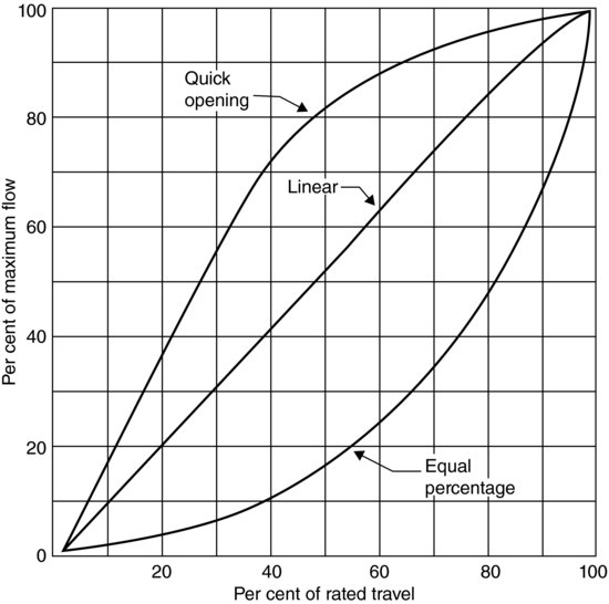
Figure 2.24 Operating characteristic for a small value of β.
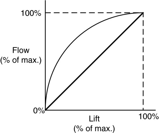
With such a characteristic as a small β, nearly full flow is obtained when the valve is opened by a small amount. Thus, the effective stem movement range for throttling flow is greatly reduced and erosion of the valve is increased since the plug is nearly closed at all flows. Therefore, a small β is undesirable and is caused by a valve that is too large. Decreasing the valve size increases the value of ΔPv (open). This, of course, increases the required pumping costs because of the extra power required to overcome the greater resistance of the valve.
Valve Selection Based on Control Performance
From the point of view of control performance, there are two aspects that need to be considered when selecting a valve. These are valve size and valve inherent characteristic.
As previously stated, these two aspects are not independent since the flow characteristics obtained depend on both. Ideally, the valve size should be decided during the design phase of the plant in conjunction with the choice of pipe and pump size. In this way, it can be ensured that the valve pressure drop is a satisfactory proportion of the total pressure drop, and thus will produce a satisfactory operating characteristic.
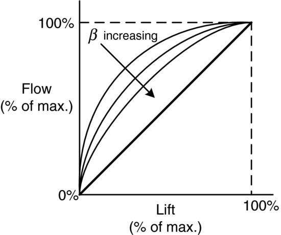
It is usually recommended that β be at least 30%. In satisfying this relationship the valve is seldom the same size as the pipe, and usually the valve will be one size smaller, with the minimum recommended size being 50% of the line size. When the control valve is added to an existing system, it is often sized to handle the maximum required flow with the available pressure drop. However, this generally results in an oversized valve since the pump was not originally designed for losses in the valve. This, in turn, then leads to a poor valve characteristic and unsatisfactory control. For this reason, an equal percentage characteristic should be selected so that the operating characteristic tends towards linear (Figure 2.25). In addition, the equal percentage characteristic is more forgiving when sized incorrectly or if there is insufficient pressure drop across the valve. Equal percentage valve plug trim has become the standard type of trim when valves are put into an existing system.
Figure 2.25 Effect of increasing the value of β.
If the control system is included as part of the original design, an equal percentage may not be the best choice, and a linear flow characteristic may also not be suitable. If the process is not linear, then the required open loop gain to obtain a given degree of stability will vary with the operating point. With a non-linear operating characteristic the valve gain will also vary with the operating point, and so it may be possible to match the valve's characteristic to that of the rest of the control system to produce roughly a constant system gain at all operating points.
This matching of the valve characteristic to that of the process is only relevant if the operating point of the process does not vary over the whole range, that is, it is not subject to large disturbances. In this case, there may be no way of matching the valve to the process if there is more than one variable that produces appreciable changes to the operating point. This is because the best characteristic for the compensation of the effects of one load variable may be different from that required for another. However, if there is only one load variable, it is often possible to determine the best shape of the valve's inherent characteristic by the use of process dynamics.
Valve Selection Based on Process Dynamics
Gain is defined as the change in output divided by the change in input. Each component in the control loop has a gain term associated with it. The control valve has a very clearly defined gain term that depends on valve type, size, pressure drop and so on. The process gain term depends upon the process response to a change in input and the various load disturbances imposed upon it. A control system should be designed such that a controller produces an effect equal to the disturbance but 180° out of phase, to bring about cancellation. Thus, for good control the loop gain should be unity as shown in Equation 2.6. If the gain is less than unity then the disturbance is not fully cancelled, and if the gain is greater than unity then the corrective action is excessive. This concept of gain is explained in greater detail in Chapter 3:
For a given set of controller settings, the controller gain and the sensor/transmitter gains may be considered as constants, resulting in the relationship of Equation 2.7:
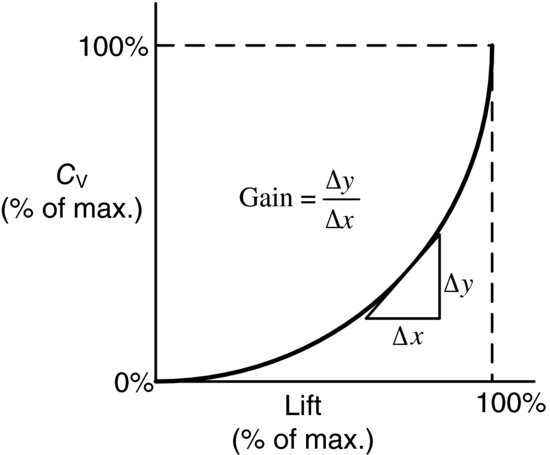
The gain of the control valve can be computed from the Cv versus lift curves as the slope of the tangent to the curve, as shown in Figure 2.26.
Figure 2.26 Calculation of the control valve gain.
If this is done for the common types of control valves over their whole range then the gain curves shown in Figure 2.27 are obtained.
Figure 2.27 Gain curves for common types of control valves.
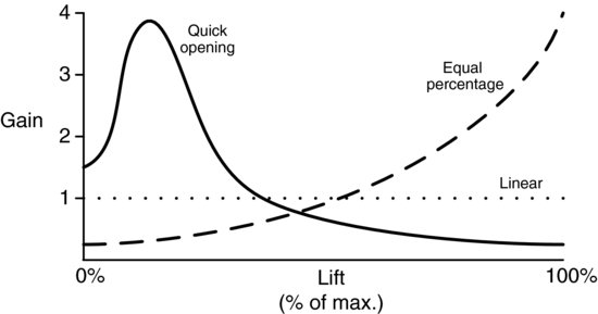
Quick Opening
The gain increases to a maximum at about 20% of the valve opening from where it decreases exponentially resulting in decreasing effectiveness as the valve approaches fully open position. This indicates that the valve would be good for a process whose gain increases with the variable used to control it.
Linear
The gain of the truly linear valve is a constant not depending on lift at all. The flow is proportional to the valve position. For example, at 50% open the flow is 50% of the maximum. This characteristic would suit a plant whose gain was independent of the operating point.
Equal Percentage
The gain increases exponentially for equal percentage lifts between 10% and 100%. This inherent characteristic is clearly best used for a process whose gain decreases as the load increases.
There are, however, rules of thumb for selecting control valves and matching inherent valve characteristics to common process control loops or processes where the valve pressure drop is fairly constant. The equal percentage characteristic is the most common and is used where variations in pressure drop are expected or in systems where a small percentage of the total system pressure drop is taken across the valve, such as in pressure and flow control. More detailed recommendations are available from control valve vendors (e.g. [18,19]).
Quantitatively, β is used to recommend a valve characteristic type. If β > 0.5, implying relatively less variation in pressure drop as the valve operates, then a linear characteristic is recommended. If β < 0.5, implying relatively more variation in pressure drop as the valve operates, then an equal percentage is recommended. Ultimately, however, valve gain is used to check the valve selection. For a selected valve, the procedure is as follows:
![]()
Control Valve Rangeability
The required range of Cv should fall between 20% and 80% of valve opening. This tends to provide a relatively constant gain and the most stable range of control. This can be checked by doing an analysis of the valve gain as discussed previously and in Purcell [22]. At less than 10% open, it can be difficult for the control valve to stabilize and it tends to oscillate, while at greater than 80% opening the gain begins to vary too much.
Control Valve Pressure Drop
Control valves control flow by absorbing a pressure drop, which must be specified. This pressure drop is an economic loss to the system since, typically, it must be supplied by a pump or compressor. As such, economics might dictate sizing a control valve with a low pressure drop, but this results in a larger valve which may have a decreased range of control. Often, the pressure drop to be taken across the control valves is specified when detailed plant hydraulics is not complete and so it needs to be estimated. As such, there are several rules of thumb. Typically, the control valve pressure drop is estimated as 50% of the friction pressure drop taken across the equipment plus piping, or 33% of the total system pressure drop (excluding the valve). Minimum pressure drops have been stated as 10% of the system pressure drop for equal percentage valves, or 25% of the system pressure drop for linear valves [23] or 35 kPa for rotary valves and 69 kPa for globe valves [22].
As stated previously, the key to sizing control valves properly is to specify the range across which they have to function. Specifying a pressure drop with the above rule of thumb at one condition means that the pressure drop required at other conditions must be checked. The required pressure drops at other conditions are governed by system hydraulics. For example, assume that we have a system pressure drop of 50 kPa. Based on taking 33% of the total system drop at design flow, excluding the valve, a pressure balance results in the control valve taking 25% of 50 kPa or 12.5 kPa while the system takes 37.5 kPa. For simplicity, assume there is no elevation component. What happens if the flow increases by 20% above the design value? Hydraulics states that the system pressure drop will increase to 72 kPa. Where is this pressure drop going to come from? The answer is the control valve but in this case we do not have sufficient pressure drop to supply it and so this system could not have an increase of 20% flow above design. The rule of thumb pressure drop should be at maximum flow and then you should check what happens at minimum flow. A more engineered approach is derived by Connell [24] with the results given in Equation 2.8. In this approach, the pressure drop across a control valve can be estimated:
where ΔPcv is the pressure drop across a control valve (kPa), Ps is the upstream or supply pressure (kPa), Qm is the maximum anticipated flow rate, Qd is the design flow rate, ΔPf is the friction pressure drop at the design flow rate (kPa) and ΔPb is the base (minimum) control valve pressure drop (kPa).
The first term accounts for a fall-off in overall system pressure drop by using 5% of the system start pressure. The second term accounts for an increase in system flow from design to maximum and the corresponding friction pressure drop. The last term is the base (minimum) control valve pressure drop from [24], given in Table 2.2.
Table 2.2 Base (minimum) pressure drops for control valve types.
| Control Valve Type | ΔPb (kPa) |
| Single plug (globe) | 75.8 |
| Double plug (globe) | 48.3 |
| Cage | 27.6 |
| Butterfly | 1.4 |
| Ball | 6.9 |
It should be noted that the values for butterfly and ball valves in Table 2.2 appear to be somewhat lower than what others recommend. As such, a minimum pressure drop of 27.6 kPa should be used unless experience indicates a specific low pressure drop application, for example, a sulphur plant air control valve.
Practical Control Valve Sizing
Note that to calculate the range of size required, the following sizing procedures require the pressure drop at minimum flow and maximum flow, not just at design flow or an arbitrary multiple thereof. However, conditions at design flow can also be incorporated and helpful. Note that the procedures use the equations developed by Fisher [18,19] but the sizing procedures are generic. In order to size a control valve properly, the following process information must be known:
- Fluid type and viscosity
- Range of controlled flows (minimum and maximum)
- Range of inlet and outlet pressures (minimum and maximum pressure drops corresponding to flows)
- Specific gravity (SG)
- Temperature
In addition, the following data need to be specified before a valve is purchased:
- Shut-off pressure
- Leakage rate (ANSI/IEC Leakage Class [17, 20])
- Noise tolerance (ANSI/IEC Standard [17, 20])
Currently manufacturers worldwide are implementing the IEC Valve Sizing Code [20]. This is a procedure that allows tighter noise prediction, particularly in gas service.
Liquid Control Valve Sizing
The basic procedure for sizing is, for a given flow rate and pressure drop, to calculate the required Cv as per a rearrangement of Equation 2.4:
This calculation should be performed at minimum and maximum conditions to obtain Cv,min and Cv,max. Subsequently, these required values are compared to a Cv range for a particular valve. Typically, the required Cv values should fall in the range of about 20–80% of the valve opening.
A plot (Figure 2.28) of Equation 2.4 implies that the relationship of flow is linear with respect to the square root of pressure drop, with the slope equal to Cv, and that the flow can be continually increased with pressure drop.
Actually, a limit is reached where this is no longer true, known as choked flow. As liquid passes through a reduced cross-sectional area, the velocity increases and the pressure decreases. The point of minimum pressure and maximum velocity is the vena contracta. As the fluid exits, the velocity is restored but the pressure is only partially restored, creating a pressure drop as shown in Figure 2.29. Note that pressure recovery is how much pressure is restored from the vena contracta. As such, all else being equal, a high recovery valve has a low pressure drop and vice versa.
Figure 2.28 Flow versus square root of the pressure drop across a control valve.
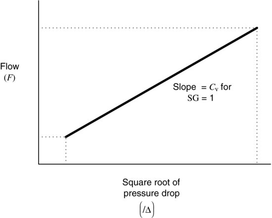
Figure 2.29 Pressure profiles across a control valve (Reproduced by permission of Emerson Process Management).

If the minimum pressure falls below the vapour pressure of the liquid, it partially vaporizes. This is what causes cavitation and flashing, discussed in more detail later. At the vena contracta, as the pressure decreases, the density of the vapour phase, and mixture, decreases. Eventually, this decrease in density offsets any increase in the velocity of the flow so that no additional mass flow is realized, according to the continuity equation.
The issue becomes how choked flow is integrated into liquid valve sizing. Fisher Controls [18,19] defines a pressure recovery coefficient as follows:
where Pvc is the pressure at the vena contracta.
Experimentally, it has been found that Pvc = rcPv, where Pv is the vapour pressure. Typically, rc is obtained from a graph, like Figure 2.30.
Figure 2.30 rc versus Pv/Pc.
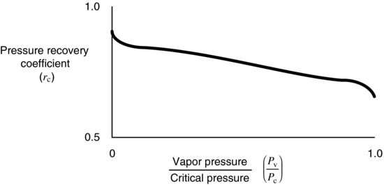
Note that water has a similar but different curve for obtaining rc. Equation 2.10 can be rearranged as
In Equation 2.11, Km is constant for a particular valve. Other control valve vendors also have an expression for ΔPallow that are functions of vapour and critical pressures. Overall, this results in the following liquid sizing procedure.
Liquid Sizing Procedure
The minimum flow often corresponds to maximum pressure drop and vice versa and these actual pressure drops are determined by system hydraulics (as discussed earlier). Also note that there are Cv corrections for viscous flow for cases where the valve Reynolds numbers are less than 5000. Finally note that the valve characteristic type and rangeability should be checked, as detailed earlier. Although sizing equations in this sections use Fisher nomenclature, they are equivalent to ANSI/ISA versions if ![]() is substituted for Km.
is substituted for Km.
Gas, Vapour and Steam Control Valve Sizing
The major differences between liquid service and gas, vapour or steam service are
- that the fluid is compressible and
- the phenomenon of critical flow.
When the ratio of ΔP/P1 exceeds 0.02, the gas is undergoing compression. Critical flow occurs when the flow is not a function of the square root of the pressure drop across the valve, but only of the upstream pressure. This phenomenon occurs when the fluid reaches sonic velocity at the vena contracta. Since gas cannot travel faster than sonic velocity, critical flow is a flow-limiting condition for gas. It has been found that critical flow occurs at different ΔP/P1 ratios, depending on whether the valve is high or low recovery.
Fisher, as well as other vendors, has equations for gas, vapour and steam flow, which have two parameters. One parameter represents flow capacity while the other parameter represents the type of valve and its effect on critical flow. The Fisher equations are as follows:
(2.12) 
(2.13) 
(2.14) 
The constant, Ca, in the denominator is 59.64 if the sine evaluation is in radians and is 3417 if the sine evaluation is in degrees and C1 = Cg/Cv.
For these equations, when ΔP / P1 ≤ 0.02 and sin(x) ≈ x, the Cg equation reduces to a ‘gas version’ of the basic equation for liquids because the pressure drop is far below the critical value and the compressibility is negligible:
(2.15) 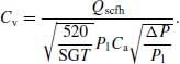
At the critical pressure drop, sin(x) ≈ 1 and Cg is only a function of P1:
(2.16) 
Overall, this results in the following gas, vapour or steam sizing procedure.
Gas, Vapour or Steam Sizing Procedure
The ANSI/ISA valve sizing equation for gas is

In Equation 2.17, Y is an expansion factor (ratio of flow coefficient for a gas to that for a liquid) that plays a similar role to C1. Although the form of this equation seems much different than the Fisher one, the results are equivalent. Again, the valve characteristic type and rangeability should be checked.
Cavitation and Flashing
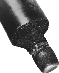
As stated previously, if the pressure in the vena contracta falls below the vapour pressure of a liquid, it will partially vaporize. If the pressure recovers above the vapour pressure, the gas bubbles collapse on the metal and tend to break it away in small pieces. This is known as cavitation (Figure 2.31). Because the pressure drop across the valve varies as the opening varies, cavitation may not occur across the entire range of valve opening. If the pressure does not recover above the vapour pressure, flashing occurs (Figure 2.32) which can erode the valve plug and seat. Fisher uses a similar equation to Equation 2.18 to describe cavitation pressure drop:
Figure 2.31 Typical appearance of flashing damage (Reproduced by permission of Emerson Process Management).
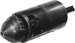
Figure 2.32 Typical appearance of cavitation damage (Reproduced by permission of Emerson Process Management).
The values for Kc are constant for a particular type of valve. Fisher has related Kc to Km, with a few examples given in Table 2.3.
Table 2.3 Kc/Km values for some valve types.
| Valve Type | Kc/Km |
| Globe valve (cavitation control trim) | 1.00 |
| Globe valve (standard trim) | 0.85 |
| Ball valve | 0.67 |
| Butterfly valve | 0.50 |
Other control valve vendors use a similar equation.
Control valves can be designed to prevent cavitation or at least minimize the damage from flashing. For example, cavitation control-type valve trims use the concept of reducing the pressure in several small increments through several stages (Figure 2.33), instead of one larger pressure drop in a single stage. This avoids the pressure in the vena contracta dropping below the liquid vapour pressure. Flashing is determined by the system, and not the control valve, because the outlet pressure is below the vapour pressure of the liquid. However, flashing damage can be minimized by using specially designed valve trims.
Figure 2.33 Multistage pressure drop (Reproduced by permission of Emerson Process Management).

Valve Positioners
Valve positioners are used to assist positioning control valves under difficult service applications where the control valve may otherwise be out of balance. Their operation employs the negative feedback principle. The position of the valve stem is balanced via cam and beam with the signal from the controller. The out-of-balance motion is detected by a nozzle, which increases the air to the top of the valve via a relay until equilibrium is obtained. Figure 2.34 illustrates the function of a pneumatic positioner for a diaphragm actuator, while Figure 2.35 shows a modern control valve utilizing a digital valve positioner.
Figure 2.34 Pneumatic positioner schematic for diaphragm actuator (Reproduced by permission of Emerson Process Management).

Valve positioners should be used when any of the following conditions apply:
- single ported valves with high pressure drops that require large stem thrusts;
- viscous liquids, sludges and slurries;
- large distances between the controller and control valve;
- three-way control valves;
- unusually tight packing required because of corrosive fluids, low emissions or high temperatures;
- large valves that use high volumes of control air; and
- split range operation, which is when two or more valves are operated by one controller.
In addition, with increasing emphasis on economic performance, valve manufacturers currently recommend that positioners be considered for valve applications where process variability performance is important [25].
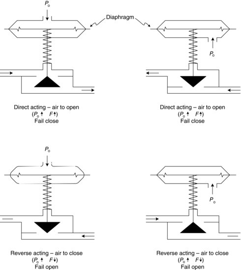
Fail-Safe Design
‘Fail-safe’ design means that if a plant has to close down because of instrument power supply failure, of either air or electricity, then the process is designed to shut down safely. This ensures safety for the environment, people, product and equipment. Fuel gas valves to fired heaters would fail closed; cooling water valves generally fail open. Several control valve designs are available that allow this purpose. The way a valve is classified is by the manner it closes under the action of the spring. There is fail-safe open- and also fail-safe close-type designs. Figure 2.36 illustrates these fail-safe designs.
Figure 2.35 Modern control valve and digital valve positioner (Reproduced by permission of Emerson Process Management).

Figure 2.36 Fail-safe design of valves.
References
1. Giacobbe, J.B. and Bounds, A.M. (1952) Selecting and working Bourdon tube materials. Instrument Manufacturing, Jul–Aug.
2. Goitein, K. (1952) A dimensional analysis approach to Bourdon tube design. Instrumentation Practice, Sep, 748–755.
3. Considine, D.M. (ed.) (1993) Process Industrial Instruments and Controls Handbook, 4th edn, McGraw-Hill.
4. Doran, C. (1997) Matching pressure transmitters. Chemical Processing, Fluid Flow Annual.
5. Kompass, E.J. (1983) SMART transmitter stores calibration digitally. Control Engineering, 30(11), 80–81.
6. Perry, R.H., Green, D.W. and Maloney, J. (1997) Perry's Chemical Engineer's Handbook, 7th edn, McGraw-Hill, pp. 8.49–8.50.
7. Parker, S. (1997) Level selection basics. Chemical Processing, Fluid Flow Annual.
8. Lieberman, N. (1977) Instrumenting a plant to run smoothly. Chemical Engineering, 84(19), 140–154.
9. Fisher Educational Services Student Guide (1991) Fundamentals of Level Measurement, Fisher Controls International Inc., USA.
10. Johnson, F.L. (1998) Temperature measurement and control fundamentals. Chemical Processing, Jun, 89–99.
11. Parker, S. (1997) Flowmeter classifications, applications and performance factors. Chemical Processing, Fluid Flow Annual.
12. ISO (1980) Standards 5167. Measurement of Fluid Flow by Means of Orifice Plates, Nozzles, and Venturi Tubes Inserted in Circular Cross-section Conduits Running Full, ISO.
13. McMillan, G.K and Considine, D.M. (eds) (1999) Process Industrial Instruments and Controls Handbook, 5th edn, McGraw-Hill.
14. Clevett, K.J. (1986) Process Analyzer Technology, John Wiley & Sons.
15. Marlin, T. McMaster University Process Control Education Website, 1999, 2000, 2001, 2005, 2009, http://www.pc-education.mcmaster.ca/Instrumentation/go_inst.htm, (accessed 4 December 2012).
16. Hauhia, M. (2000) Control Fundamentals: A Primer for Graduates…A Refresher Course for Experienced Engineers, InTech, Oct, pp. 69–71.
17. ANSI/ISA Standard S75.01. Control Valve Sizing Equations (revised periodically). ISA, Research Triangle Park, NC.
18. Control Valve Handbook. (1998) 3rd edn, Fisher Controls International Inc., USA.
19. Control Valve Sourcebook, Power A Severe Service. (1990) 2nd edn, Fisher Controls International, Inc., USA.
20. IEC (1995) 534-8-3. Control Valve Standard.
21. Masoneilan (1981) Handbook for Control Valve Sizing. Bull. OZ-100, Masoneilan Division, McGraw-Edison Co., Norwood, MA.
22. Purcell, M.K. (1999) Easily select and size control valves. CEP, 45–50.
23. Bell, R.M. (1996) Avoid pitfalls when specifying control valves. Chemical Engineering, Dec, 75–77.
24. Connell, J.R. (1987) Realistic control valve pressure drops. Chemical Engineering, Sep(28), 123–127.
25. Rheinhart, N.F. (1997) Impact of control loop performance on process profitability, Aspen World ‘97, Boston, MA, USA, 15 October 1997.