1

A Brief History of Process Control and Process Simulation

In order to gain an appreciation for process control and process simulation it is important to have some understanding of the history and motivation behind the development of both process control and process simulation. Rudimentary control systems have been used for centuries to help humans use tools and machinery more efficiently, effectively and safely. However, only in the last century has significant time and effort been devoted to developing a greater understanding of controls and sophisticated control systems, a requirement of the increased complexity of the processes to be controlled. The expansion of the controls field has driven the growth of steady-state and dynamic process simulation from relative obscurity to the indispensable and commonplace tool that it is today, in particular in the development of operator training systems and the validation of complex control strategies.

1.1 Process Control

Feedback control can be traced back as far as the early third century BC [1,2]. During this period, Ktesibios of Alexandria employed a float valve similar to the one found in today's automobile carburettors to regulate the level in the water clocks of that time [3]. Three centuries later, Heron of Alexandria described another float valve water level regulator similar to that used in toilet water tanks [1]. Arabic water clock builders used this same control device as late as 1206. The Romans also made use of this first control device in regulating the water levels in their aqueducts. The level-regulating device or float valve remained unknown to Europeans and was reinvented in the eighteenth century to regulate the water levels in steam boilers and home water tanks.

The Europeans did, however, invent a number of feedback control devices, namely the thermostat or bimetallic temperature regulator, the safety relief valve, and the windmill fantail. In 1620, Cornelis Drebbel [3], a Dutch engineer, used a bimetallic temperature regulator to control the temperature of a furnace. Denis Papin [3], in 1681, used weights on a pressure cooker to regulate the pressure in the vessel. In 1745, Edmund Lee [1] attached a fantail at right angles to the main sail of a windmill, thus always keeping the main windmill drive facing into the wind. It was not until the Industrial Revolution, particularly in England, that feedback devices became more numerous and varied.

One-port automata (open loop) evolved as part of the Industrial Revolution and focused on a flow of commands that mechanized the functions of a human operator. In 1801, Joseph Farcot [4] fed punched cards past a row of needles to program patterns on a loom, and in 1796, David Wilkinson [5] developed a copying lathe with a cutting tool positioned by a follower on a model. Oliver Evans [3] built a water-powered flourmill near Philadelphia, in 1784, using bucket and screw conveyors to eliminate manual intervention. Similarly, biscuit making was automated for the Royal Navy in 1833, and meat processing was mechanized in America during the late 1860s. Henry Ford used the same concept for his 1910 automobile assembly plant automation. Unit operations, pioneered by Allen Rogers of the Pratt Institute [5] and Arthur D. Little of MIT [5], led to continuous chemical processing and extensive automation during the 1920s.

The concept of feedback evolved along with the development of steam power and steam-powered ships. The valve operator of Humphrey Potter [6] utilized piston displacement on a Newcomen engine to perform a deterministic control function. However, the fly ball governor designed by James Watt [7] in 1769 modulated steam flow to overcome unpredictable disturbances and became the archetype for single-loop regulatory controllers. Feedback was accompanied by a perplexing tendency to overshoot the desired operating level, particularly as controller sensitivity increased. The steam-powered steering systems of the ships of the mid-1800s used a human operator to supply feedback, but high rudder positioning gain caused the ship to zigzag along its course. In 1867, Macfarlane Gray [1] corrected the problem with a linkage that closed the steering valve as the rudder approached the desired set point. In 1872, Leon Farcot [1] designed a hydraulic system such that a displacement representing rudder position was subtracted from the steering position displacement, and the difference was used to operate the valve. The helmsman could then indicate a rudder position, which would be achieved and maintained by the servo motor.

Subsequent refinements of the servo principle were largely empirical until Minorsky [8], in 1922, published an analytical study of ship steering which considered the use of proportional, derivative and second derivative controllers for steering ships and demonstrated how stability could be determined from the differential equations. In 1934 Hazen [9] introduced the term ‘servomechanism’ for position control devices and discussed the design of control systems capable of close tracking of a changing set point. Nyquist [10] developed a general and relatively simple procedure for determining the stability of feedback systems from the open loop response, based on a study of feedback amplifiers.

Experience with and the theories of mechanical and electrical systems were, therefore, available when World War II created a massive impetus for weapon controls. While the eventual social benefit of this and subsequent military efforts is not without merit, the nature of the incentives emphasizes the irony seen by Elting Morison [11]. Just as we attain a means of ‘control over our resistant natural environment we find we have produced in the means themselves an artificial environment of such complexity that we cannot control it’.

Although the basic principles of feedback control can be applied to chemical processing plants as well as to amplifiers or mechanical systems, chemical engineers were slow to adapt the wealth of control literature from other disciplines for the design of process control schemes. The unfamiliar terminology was one major reason for the delay, but there was also the basic difference between chemical processes and servomechanisms, which delayed the development of process control theory and its implementation. Chemical plants normally operate with a constant set point, and large-capacity elements help to minimize the effect of disturbances, whereas these would tend to slow the response of servomechanisms. Time delay or transport lag is frequently a major factor in process control, yet it is rarely mentioned in the literature on servomechanisms. In process control systems, interacting first-order elements and distributed resistances are much more common than second-order elements found in the control of mechanical and electrical systems. These differences made many of the published examples of servomechanism design of little use to those interested in process control.

A few theoretical papers on process control did appear during the 1930s. Notable among these was the paper by Grebe, Boundy and Cermak [12] that discussed the problem of pH control and showed the advantages of using derivative action to improve controller response. Callender, Hartree, and Porter [13] showed the effect of time delay on the stability and speed of response of a control system. However, it was not until the mid-1950s that the first texts on process control were published by Young, in 1954 [14], and Ceaglske, in 1956 [15]. These early classical process control texts used techniques that were suitable prior to the availability of computers, namely frequency response, Laplace transforms, transfer function representation and linearization. Between the late 1950s and the 1970s many texts appeared, generally following the pre-computing classical approach, notably those by Eckman [16], Campbell [17], Coughanowr and Koppel [18], Luyben [19], Harriott [20], Murrill [21] and Shinskey [22]. Process control became an integral part of every chemical engineering curriculum.

Present-day process control texts that include Marlin [23], Seborg et al. [24], Smith [25], Smith and Corripio [26], Riggs [27] and Luyben and Luyben [28] have to some extent used a real-time approach via modelling of the process and its control structure using MATLAB Simulink [29] and Maple [30] to provide a solution to the set of differential equations, thus viewing the real-time transient behaviour of the process and its control system.

A book by King [31] titled Process Control: A Practical Approach is aimed at the practising controls engineer. It, like this text, focuses on the practical aspects of process control. This book is an excellent addition to the practising controls engineer's library.

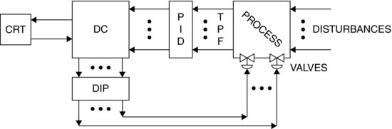
The availability of minicomputers in the late 1950s and early 1960s provided the impetus for the use of these computers for centralized process control (DC). For instance the IBM 1800 of that time was equipped with a hardware interface that could convert measured temperatures, flows and so on (analog signals) to the required digital signals (PID). A number of early installations were only digital computer-based data loggers (Figure 1.1). The first computer-based central control system [2] was installed in 1959 at the Texaco Port Arthur, Texas refinery, and was based on an RW-300 from Ramo-Woolridge (Figure 1.2). During the following decade a number of centralized digital control systems were installed in chemical plants and refineries [32]. These installations for the most part were supervisory (Figure 1.3) because these facilities could not risk a digital computer failure without a conventional reliable single-loop control structure as a back-up.

Figure 1.1 Digital computer-based data logger of the late 1950s and 1960s.

Figure 1.2 Schematic of centralized digital computer control structures.

In 1975, both Honeywell and Yokogawa provided the first distributed control system (DCS) [2] (Figure 1.4). Over the next decade virtually all the control hardware providers developed and offered a DCS.

Figure 1.3 Schematic of supervisory digital control systems of the 1970s.

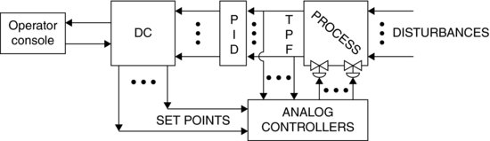
Figure 1.4 Schematic of a modern distributed control system (DCS).

The fluid-processing industries quickly adopted this combination of hardware and software. This approach to process control offered a natural extension to the typical process/plant SISO control loops. The plant controllers and measurements were not centrally located but ‘distributed’ throughout the plant. Hence, basic control is achieved at the local loop level. These local controllers and local measurements are then connected via a communication network for monitoring and display to a central control room. A central aspect of the current DCSs is the quality and detail of the plant equipment hardware displays, the process measured and controlled variable displays.

Figure 1.2 is a schematic of a centralized digital control structure while Figure 1.4 shows the structure of a typical DCS. The obvious difference is the distribution of controllers as groups of digital controllers, that is, only the key loops are backed up with a SISO loop. The DCS has the major advantage that even if the central processor should fail the underlying control system continues to function.

DCS hardware will be discussed further in Chapter 2. DCS software has developed to the point of providing advanced control strategies such as MPC and DMC, detailed graphic displays and user programming capability – in other words, very operator friendly.

1.2 Process Simulation

Prior to the 1950s, calculations had been done manually1 on mechanical or electronic calculators. In 1950, Rose and Williams [33] wrote the first steady-state, multistage binary distillation tower simulation program. The total simulation was written in machine language on an IBM 702, a major feat with the hardware of the day. The general trend through the 1950s was steady-state simulation of individual units. The field was moving so rapidly that by 1953 the American Institute of Chemical Engineers (AIChE) had the first annual review of Computers and Computing in Chemical Engineering. The introduction of FORTRAN by IBM in 1954 provided the impetus for the chemical process industry to embrace computer calculations. The 1950s can be characterized as a period of discovery [34].

From the early 1960s to the present day, steady-state process simulation has moved from a tool used only by experts to a software tool used daily to perform routine calculations. This was made possible by the advances in computing hardware, most significant of which has been the proliferation of powerful desktop computers [personal computers (PCs)], the development of Windows-based systems software and the development of object-oriented programming languages. This combination of inexpensive hardware and system tools has led to the proliferation of exceptionally user-friendly and robust software tools for steady-state process simulation and design. Dynamic simulation naturally developed along with the steady-state simulators [35]. Figure 1.5 presents a summary of the growth of dynamic process simulation.

Figure 1.5 Development of dynamic process simulators.

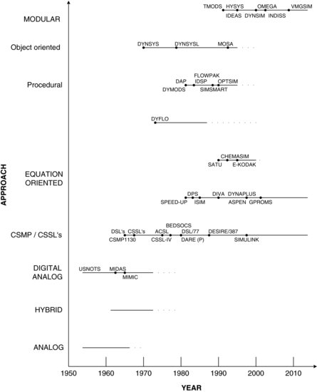
During the 1960s, the size of the analog computer controlled the size of the simulation. These analog computers grew from a few amplifier systems to large systems of a hundred or more amplifiers and finally in the late 1960s to hybrid computers [36]. It was recognized very early that the major disadvantages of analog computers were problem size and dynamic range, both of which were limited by hardware size. Hybrid computers were an attempt to mitigate some of these problems. However, hybrid computers of the late 1960s and early 1970s still had the following problems that limited their general acceptance [36]:

Engineers were searching for a dynamic simulator that paralleled steady-state simulators being developed during the late 1960s and early 1970s. Early attempts simply moved the analog to a digital formation (CSMPs, Pactolus, etc.) by providing numerical integration algorithms and a suitable programming syntax. Latter versions of these block-oriented dynamic simulators provided more functionality and an improved programming methodology. This approach resulted in various continuous system simulation languages (CSSLs) of which ACSL [37] is the most widely used.

Parallel to the previous approach has been the development of equation-based numerical solvers like SPEEDUP [38]. These tools are aimed at the specialist who has considerable experience in using the tool, knows how to model various processes in terms of their fundamental equations and is willing to spend considerable time entering code and data into input files, which are compiled, edited and debugged before they yield results of time plots for selected variables over fixed time periods. These equation-based dynamic simulation packages were very much the realm of the expert. Concepts such as ease of use, complex thermodynamic packages and libraries of reusable unit operations had not migrated to these dynamic simulators.

The first attempts to provide a modular-based dynamic process simulator were made by Franks and Johnson [39]. The two early modular simulators, DYFLO and DYNSYS, differed in their approach. DYFLO provided the simulator with a suite of FORTRAN routines that were linked via a program written by the user. Hence, it was to some extent cumbersome, but useable. DYNSYS [39], on the other hand, provided a key word structure much like the steady-state simulators of the era allowing the user to build a dynamic simulation. Both simulators found limited use due to the difficulty of producing a simulation and the actual run times on the computer hardware of the time were often greater than real time.

During the late 1970s and throughout the 1980s only equation-oriented simulators were used. There was a continuing effort to develop and extend dynamic models of plants and use these for control system development. Many companies, from necessity, had groups using this approach to develop specific plant dynamic simulations and subsequently using these simulations for control design and evaluation. Marquardt at CPCIV [40] in 1991 presented a paper summarizing key developments and future challenges in dynamic process simulation. Since this review three additional dynamic process simulators have appeared – Odysseo [41], Ideas [42] and VMGSim [43].

The key benefits of dynamic simulation [44] are related to the improved process understanding that it provides; plants are, by their nature, dynamic. By understanding the process more fully, several benefits follow naturally. These include improvements in control system design, improvements in the basic operation of the plant, and improvements in training for both operators and engineers.

Control system design is, unfortunately, still often left until the end of the design cycle. This practice frequently requires an elaborate control strategy in order to make the best of a poor design. Dynamic simulation, when involved early in the design phase, can help to identify the important operability and control issues and influence the design accordingly. Clearly, the ideal is not just to develop a working control strategy, but also to design a plant that is inherently easy to control.

Using a rigorous dynamic model, control strategies can be designed, tested and even tuned prior to start-up. With appropriate hardware links, dynamic models may even be used to checkout DCS or other control system configurations. All of these features make dynamic simulation ideally suited to control applications.

Another benefit involves reconciling trade-offs between steady-state optimizations and dynamic operability. To minimize capital expenditures and operating utility costs, many plant designers have adopted the use of steady-state optimization techniques. As a result, plant designs have become more complex and much more highly integrated and interactive. Examples include extensive heat exchange networks, process recycles, and minimum hold-up designs. While such designs may optimize the steady-state flowsheet, they present particular challenges to plant control and operations engineers, usually requiring advanced control strategies and a well-trained operating staff. This trade-off between steady-state optimization and dynamic operability is classic and can only be truly reconciled using dynamic simulation.

Once a plant is in operation, manufacturing personnel are continually looking for ways to improve quality, minimize waste, maximize yield, reduce utility costs and often increase capacity. It is in this area of process improvements where dynamic simulation has, perhaps, the most value-adding impact. This is also the area where it is most important to minimize the usage barriers for dynamic simulation. Since plant-operating personnel are typically busy with the day-to-day operation of the plant, simulation tools that are difficult to understand and use will never see any of the truly practical and value-adding applications. By allowing plant engineers to quickly and easily test theories, illustrate concepts or compare alternative control strategies or operating schemes, dynamic simulation can have a tremendous cumulative benefit.

Over the past several years, the industry has begun to focus a great deal of attention and interest on dynamic simulation for training purposes. As mentioned earlier, the increased complexity of the plants being designed today requires well-trained operating personnel (OTS). In order to be effective, the training simulator should be interactive, be realistic and run real time. By running a relatively high-fidelity model, operators can test ‘what if’ scenarios, practice start-up and shutdown sequences and respond to failure and alarm situations.

More recently, training simulators have provided links to a variety of DCS platforms. By using the actual control hardware to run a dynamic model of the plant, operators have the added benefit of training on the same equipment that will be used to operate the real process.

It is important at this point to introduce the notion of breadth of use for a model. We have discussed the use of dynamic simulation for design, control, operations and, now, training. Indeed, it would be beneficial if the same model used to design the plant, develop its controls and study its operation could be used as the on-line training simulator for DCS. While this may seem obvious, it is difficult to find examples of such applications. This is primarily due to the absence of commercial simulation tools that provide sufficient breadth of functionality – both engineering functionality and usability.

With all of the benefits to dynamic simulation, why is it that this technology has only begun to see more widespread use recently? To answer this question, it is helpful to continue with the history of simulation and to consider the unique set of skills required to develop a dynamic simulation from first principles.

First, an understanding of and access to the basic data relating to the physical properties of the chemical system is needed. This includes the vapour–liquid equilibrium (VLE) and any reaction equations involved. Second, a detailed understanding of the heat and material balance relationships in the process equipment is required. Third, knowledge of appropriate numerical techniques to solve the sets of differential and algebraic equations is needed. Finally, experience in striking a balance between rigour and performance is needed in order to build a model that is at the same time useful and useable. Thus there is indeed a unique set of skills required to design a first-principles dynamic simulator.

Because of the computational load, dynamic simulations have been reserved for large mainframe or minicomputers. An unfortunate feature of these large computer systems was their often cumbersome user interfaces. Typically, dynamic simulations were run in a batch mode where the model was built with no feedback from the program, then submitted to the computer to be solved for a predetermined length of simulation time. Only when the solution was reached could the user view the results of the simulation study.

With this approach, 50–80% of the time dedicated to a dynamic study was consumed in the model-building phase. Roughly 20% was dedicated to running the various case studies and 10% to documentation and presentation of results. This kind of cycle made it difficult for a casual user to conduct a study or even to run a model that someone else had prepared. While the batch-style approach consumed a disproportionate amount of time setting up the model, the real drawback was the lack of any interaction between the user and the simulation. By preventing any real interaction with the model as it is being solved, batch-style simulation sessions are much less effective. Additionally, since more time and effort are spent building model structures, submitting and waiting for batch input runs, a smaller fraction of time is available to gain the important process understanding through ‘what if’ sessions.

Thus, between the sophisticated chemical engineering, thermodynamics, programming and modelling skills, the large and expensive computers and cumbersome and inefficient user interfaces, it is not surprising that dynamic simulation has not enjoyed widespread use. Normally, only the most complex process studies and designs justified the effort required to develop a dynamic simulation. We believe that the two most significant factors in increased use of dynamic simulation are [35]

• the growth of computer hardware and software technology and
• the emergence of new ways of packaging simulation.

As indicated previously, there has been a tremendous increase in the performance of PCs accompanied by an equally impressive drop in their prices. For example, it is not uncommon for an engineer to have a PC with memory of upwards of 8 GB, a 512 GB hard drive, and a large flat-screen graphics monitor on his desktop costing less than $1000. Furthermore, a number of powerful and interactive window environments have been developed for the PC and other inexpensive hardware platforms. Windows (2000, NT, XP, VISTA, 7, 8, etc.), X-Windows and Mac Systems are just some examples.

The growth in the performance and speed of the PC has made the migration of numerically intense applications to PC platforms a reality. This, combined with the flexibility and ease of use of the window environments, has laid the groundwork for a truly new and user-friendly approach to simulation.

There are literally thousands of person-years of simulation experience in the industry. With the existing computer technology providing the framework, there are very few reasons why most engineers should have to write and compile code in order to use dynamic simulation. Model libraries do not provide the answer since they do not eliminate the build–compile–link sequence that is often troublesome, prone to errors and intimidating to many potential users. Given today's window environments and the new programming capabilities that languages such as object-oriented C++ provide, there is no need for batch-type simulation sessions.

It is imperative that a dynamic simulation is ‘packaged’ in a way that makes it easy to use and learn, yet still be applicable to a broad range of applications and users. The criteria include the following:

• Easy to use and learn – must have an intuitive and interactive, graphical environment that involves no writing of code or any compile–link–run cycle.
• Configurable – must provide reusable modules which can easily be linked together to build the desired model.
• Accurate – must provide meaningful results.
• Fast – must strike a balance between rigour and performance so as not to lose the interactive benefits of simulation.
• Broadly applicable – must provide a broad range of functionality to span different industrial applications, as well as varying levels of detail and rigour.
• Desktop computer based – must reside on a convenient desktop computer environment such as a PC, Mac or workstation.

With these attributes, dynamic simulation becomes not only available, but also attractive to a much larger audience than ever before. While dynamic simulation is clearly a valuable tool in the hands of seasoned modellers, only when process engineers, control engineers and plant-operating personnel feel comfortable with it will dynamic simulation deliver its most powerful and value-adding benefits.

Even with this emphasis on control system design, chemical plant design used the results of steady-state performance to size the equipment while heuristic methods rather than dynamic systems analysis chose the control schemes. Instruments were field adjusted to give performance as good as or better than manual control. When the control schemes, sensing devices, valves and the process itself produced poor results, trial and error was used to find an acceptable level of performance. The lengthy analysis required for an accurate control system design using the equation-based approach could not be justified, or was justified for very few critical loops. Vogel [45] states that even as late as 1991, only the most challenging and troublesome processes were modelled dynamically with the aim of developing process dynamic behaviour understanding and testing alternative control configurations.

For complex processes that required close control, the weakest link in the control scheme design was usually the dynamic description or model of the process. The response of the sensor, valve and controller could easily be modelled to within 5%. The modelling error in predicting the dynamic behaviour of the process was generally two to three times greater. The lack of reliable, robust, reusable dynamic process models and suitable software [46] limited the acceptance and use of process control theory. However, this situation was changed during the early 1990s with the availability of commercial robust high-fidelity process dynamic simulators and has led to the frequent use of this software tool. The vendors and a book by Luyben [47] do provide a number of examples and guidelines for the development of useful process dynamic simulations.

In summary, the traditional approach to control loop analysis has been through the use of frequency domain techniques such as Bode diagrams, transfer functions and Nyquist plots. Most of these analysis methods require a working knowledge of Laplace transforms and were developed as pencil and paper techniques for solving linear sets of different equations. Although these frequency domain techniques are useful for single control loops they are not easily applicable to real multi-loop and nonlinear systems which comprise the actual plants that must be controlled in the fluid-processing industries.

In the real-time4 approach the same set of algebraic and differential equations are encountered as in the frequency domain. However, the major advantage of solving these equations in real time is the ability to observe the interactions of the process, control scheme and load variables much as the operator of a plant observes the behaviour of an actual plant. Dynamic simulation allows for the comparison of several candidate control strategies and assesses the propagation of variation through a process/plant. In other words, dynamic simulation allows for the evaluation of plant-wide versus single-loop control schemes.

References

1. Mayr, O. (1971) Feedback Mechanisms: In the Historical Collections of the National Museum of History and Technology, Smithsonian Institution Press, City of Washington, p. 96.

2. Stout, T.M. and Williams, T.J. (1995) Pioneering work in the field of computer process control. IEEE Annals of the History of Computing, 17(1): 6–18.

3. Mayr, O. (1970) The Origins of Feedback Control, Cambridge, Massachusetts.

4. Williams, T.I. (1987) The History of Invention: From Stone Axes to Silicon Chips, MacDonald & Co. Ltd, pp. 148–161.

5. Woodbury, R.S. (1972) Studies in the History of Machine Tools, M.I.T. Press, pp. 90–93.

6. Hougen, O.A. (1977) Seven decades of chemical engineering. Chemical Engineering Progress, 73, 89–104.

7. Bennett, S. (1975) The Search for ‘Uniform and Equable Motion’: a study of the early methods of control of the steam engine. International Journal of Control, 21, 115–116.

8. Minorsky, N. (1922) Directional stability of automatically steered bodies. Journal of American Society of Naval Engineers, 34, 280.

9. Hazen, H.L. (1934) Theory of servomechanisms. Journal of the Franklin Institute, 218, 279.

10. Nyquist, H. (1932) Regeneration theory. Bell System Technical Journal, 11, 126.

11. Krigman, A. (1970) ICON, the Helmsman. Instruments and Control Systems, Dec., 4.

12. Grebe, J.J., Boundy, R.H. and Cermak, R.W. (1933) The control of chemical processes. Transactions of the American Institute of Chemical Engineers, 29, 211.

13. Callender, A., Hartree, D.R. and Porter, A. (1936) Time lag in a control system – I. Philosophical Transactions of the Royal Society of London. Series A, Mathematical and Physical Sciences, 235, 415.

14. Young, A.J. (1954) Process Control, Instruments Publishing Company, Pittsburgh.

15. Ceaglske, N.H. (1956) Automatic Process Control for Chemical Engineers, John Wiley & Sons.

16. Eckman, D. (1958) Automatic Process Control, John Wiley & Sons, New York.

17. Campbell, D.P. (1958) Process Dynamics, John Wiley & Sons, New York.

18. Coughanowr, D.R. and Koppel, L.B. (1965) Process System Analysis and Control, McGraw-Hill.

19. Luyben, W.L. (1973) Process Modeling, Simulation, and Control for Chemical Engineers, McGraw-Hill, New York.

20. Harriott, P. (1964) Process Control, McGraw-Hill, New York.

21. Murrill, P.W. (1967) Automatic Control of Processes, International Textbook.

22. Shinskey, F.G. (1967) Process Control Systems, McGraw-Hill.

23. Marlin, T.E. (2000) Process Control; Designing Processes and Control Systems for Dynamic Performance, 2nd edn, McGraw-Hill.

24. Seborg, D.E., Edgar, T.F., Mellichamp, D.A. and Doyle, F.J. (2011) Process Dynamics and Control, 3rd edn, Wiley.

25. Smith, C.L. (2010) Advanced Process Control: Beyond Single Loop Control, Wiley.

26. Smith, C.A. and Corripio, A.B. (2006) Principles and Practise of Automatic Control, Wiley.

27. Riggs, J.B. (1999) Chemical Process Control, Ferret Publishing.

28. Luyben, M.L. and Luyben, W.L. (1997) Essentials of Process Control, McGraw-Hill.

29. MATLAB Simulink http://www.mathworks.com/products/simulink/ (accessed 20 August 2013).

30. MAPLE www.maplesoft.com/ (accessed 20 August 2013).

31. King, M. (2010) Process Control: A Practical Approach, Wiley.

32. Smith, C.L. (1972) Digital Computer Process Control, Intext Educational Publishers.

33. Rose, A. and Williams, T.J. (1950) Punched card devices for distillation calculations. Industrial and Engineering Chemistry, 42, 2494.

34. Lacey, J.W. and Svrcek, W.Y. (1990) Computers and Chemical Engineers. Presented at 40th Canadian Chemical Engineering Conference, Halifax, NS, Canada.

35. Svrcek, W.Y., Sim, W.D. and Satyro, M.A. (1996) From Large Computers and Small Solutions to Small Computers and Large Solutions. Proceedings of Chemeca ‘96, Sydney, Australia, vol. 2, pp. 11–18.

36. Svrcek, W.Y. and Sandholm, D.P. (1971) An experience in the selection of a computer simulation technique. Simulation, 17(6), 245–246.

37. Strauss, J.C. et al. (1967) The SCi Continuous System Simulation Language (CSSL). Simulation, 9(6), 281–292.

38. Perkins, J.D. (1986) Survey of existing systems for the dynamic simulation of industrial processes. Modeling, Identification, and Control, 7, 71–81.

39. Ausain, A. (1986) Chemical Process Simulation, John Wiley & Sons, New York, pp. 201.

40. Marquardt, W. (1991) Dynamic process simulation – recent progress and future challenges, in Proceedings of CPCIV (eds Y. Arkun and W.H. Ray), AIChE, New York, pp. 131–180.

41. Odysseo, http://www.prosim.net/ (accessed 20 August 2013).

42. Ideas, http://www.ideas-simulation.com/ (accessed 20 August 2013).

43. VMGSim Dynamics, http://www.virtualmaterials.com/vmgsimdynamics (accessed 20 August 2013).

44. Fruehauf, P.S. and Mahoney, D.P. (1994) Improve distillation column control design. CEP, March, 75–83.

45. Vogel, E.F. (1991) An industrial perspective on dynamic flowsheet simulation, in Proceedings of CPCIV (eds Y. Arkun and W.H. Ray), AIChE, New York, pp. 181–208.

46. Tyreus, B.D. (1992) Object-oriented simulation, Chapter 5, in Practical Distillation Control (ed. W.L. Luyben), Van Nostrand Reinhold.

47. Luyben, W.L. (2002) Plantwide Dynamic Simulators in Chemical Processing and Control, Marcel Dekker, Inc.

1 Using a slide rule.

2 One week or more.

3 Human nature.

4 Time domain dynamics.