
CHAPTER 11
PRINCIPLES OF LEAST SQUARES
11.1 INTRODUCTION
![]() In surveying, observations must often satisfy established numerical relationships known as geometric constraints. As examples, in a closed-polygon traverse, horizontal angle and distance observations should conform to the geometric constraints given in Section 8.4, and in a differential leveling loop, the elevation differences should sum to given a quantity. However, because the geometric constraints rarely meet perfectly, an adjustment of the data is performed.
In surveying, observations must often satisfy established numerical relationships known as geometric constraints. As examples, in a closed-polygon traverse, horizontal angle and distance observations should conform to the geometric constraints given in Section 8.4, and in a differential leveling loop, the elevation differences should sum to given a quantity. However, because the geometric constraints rarely meet perfectly, an adjustment of the data is performed.
As discussed in earlier chapters, errors in observations conform to the laws of probability; that is, they follow normal distribution theory. Thus, they should be adjusted in a manner that follows these mathematical laws. While the mean has been used extensively throughout history, the earliest works on least squares started in the late eighteenth century. Its earliest application was primarily for adjusting celestial observations. Laplace first investigated the subject and laid its foundation in 1774. The first published article on the subject, titled “Méthode des Moindres Quarrés” (Method of Least Squares), was written in 1805 by Legendre. However, it is well known that although Gauss did not publish until 1809, he developed and used the method extensively as a student at the University of Göttingen beginning in 1794, and thus is given credit for the development of the subject. In this chapter, equations for performing least squares adjustments are developed, and their uses are illustrated with several examples.
11.2 FUNDAMENTAL PRINCIPLE OF LEAST SQUARES
To develop the principle of least squares, a specific case will be considered. Suppose there are n independent equally weighted measurements, z1, z2,…, zn, of the same quantity z that has a most probable value denoted by M. By definition,

In Equation (11.1) the v's are the residual errors. Note that residuals behave in a manner similar to errors, and thus they can be used interchangeably in the normal distribution function given by Equation (3.2). By substituting v for x, there results

where ![]() and
and ![]() .
.
As discussed in Chapter 3, probabilities are represented by areas under the normal distribution curve. Thus, the individual probabilities for the occurrence of residuals v1, v2,…, vn are obtained by multiplying their respective ordinates y1, y2,…, yn by some infinitesimally small increment of v, which is denoted as Δv. The following probability statements result

From Equation (3.1), the probability of the simultaneous occurrence of all the residuals v1 through vn is the product of the individual probabilities, and thus
Simplifying Equation (11.4) yields
M is a quantity that is to be selected in such a way that it gives the greatest probability of occurrence; stated differently, the value of M that maximizes the value of P. In Equation (11.5), the values of K, h, and Δv are all constants, and thus only the residuals can be modified by selecting different values for M. Figure 11.1 shows a plot of the e−x versus x. From this plot it is readily seen that e−x is maximized by minimizing x, and thus in relation to Equation (11.5), the probability P is maximized when the quantity ![]() is minimized. In other words, to maximize P, the sum of the squared residuals must be minimized. Equation (11.6) expresses the principle of least squares.
is minimized. In other words, to maximize P, the sum of the squared residuals must be minimized. Equation (11.6) expresses the principle of least squares.

FIGURE 11.1 Plot of e−x.
This condition states: “The most probable value (MPV) for a quantity obtained from repeated observations of equal weight is the value that renders the sum of the squared residuals a minimum.” From calculus, the minimum value of a function can be found by taking its first derivative and equating the resulting function with zero. That is, the condition stated in Equation (11.6) is enforced by taking the first derivative of the function with respect to the unknown variable M and setting the results equal to zero. Substituting Equation (11.1) into Equation (11.6) yields
Taking the first derivative of Equation (11.7) with respect to M and setting the resulting equation equal to zero yields

Now dividing Equation (11.8) by 2 and simplifying yields

In Equation (11.9) the quantity ![]() is the mean of the observed values. This is proof that when a quantity has been observed independently several times, the MPV is the arithmetic mean.
is the mean of the observed values. This is proof that when a quantity has been observed independently several times, the MPV is the arithmetic mean.
11.3 THE FUNDAMENTAL PRINCIPLE OF WEIGHTED LEAST SQUARES
In Section 11.2, the fundamental principle of a least squares adjustment was developed for observations having equal or unit weights. The more general case of least squares adjustment assumes that the observations have varying degrees of precision and thus varying weights.
Consider a set of measurements ![]() having relative weights
having relative weights ![]() and residuals
and residuals ![]() . Denote the weighted MPV as M. As in Section 11.2, the residuals are related to the observations through Equations (11.1), and the total probability of their simultaneous occurrence is given by Equation (11.5). However, notice in Equation (11.2) that
. Denote the weighted MPV as M. As in Section 11.2, the residuals are related to the observations through Equations (11.1), and the total probability of their simultaneous occurrence is given by Equation (11.5). However, notice in Equation (11.2) that ![]() , and since weights are inversely proportional to variances, they are directly proportional to h2. Thus, Equation (11.5) can be rewritten as
, and since weights are inversely proportional to variances, they are directly proportional to h2. Thus, Equation (11.5) can be rewritten as
To maximize P in Equation (11.10), the negative exponent must be minimized. To achieve this, the sum of the products of the weights times their respective squared residuals must be minimized. This is the condition imposed in a weighted least-squares adjustment. The condition of weighted least-squares adjustment in equation form is
Substituting the values for the residuals given in Equation (11.1) into Equation (11.11) yields
The condition for a weighted least square adjustment is: The most probable value for a quantity obtained from repeated observations having various weights is that value that renders the sum of the weight times their respective squared residual a minimum.
The minimum condition is imposed by differentiating Equation (11.12) with respect to M and setting the resultant equation equal to zero. This yields
Dividing Equation (11.13) by 2 and rearranging results in
Rearranging Equation (11.14a) yields
Equation (11.14b) can be written as ![]() . Thus,
. Thus,

Notice that Equation (11.15) is the same as Equation (10.13), which is the formula for computing the weighted mean.
11.4 THE STOCHASTIC MODEL
The determination of variances, and subsequently the weights of the observations, is known as the stochastic model in a least squares adjustment. In Section 11.3, the inclusion of weights in the adjustment was discussed. It is crucial to the adjustment to select a proper stochastic (weighting) model since, as was discussed in Section 10.1, the weight of an observation controls the amount of correction it receives during the adjustment. However, development of the stochastic model is important to more than the weighted adjustments. When doing an unweighted adjustment, all observations are assumed to be of equal weight, and thus the stochastic model is created implicitly. The foundations for selecting a proper stochastic model in surveying were established in Chapters 7 to 10. It will be shown in Chapter 21 that failure to select the stochastic model properly will also affect one's ability to isolate blunders in observational sets.
11.5 FUNCTIONAL MODEL
A functional model in adjustment computations is an equation or set of equations/functions that represents or defines an adjustment condition. It must either be known or assumed. If the functional model represents the physical situation adequately, the observational errors can be expected to conform to the normal distribution curve. For example, a well-known functional model states that the sum of angles in a triangle is 180°. This model is adequate if the survey is limited to a small region. However, when the survey covers very large areas, this model does not account for the systematic errors caused by curvature of the Earth. In this case, the functional model is inadequate and needs to be modified to include corrections for spherical excess. In traversing, the functional model of plane computations is suitable for smaller surveys, but if the extent of the survey becomes too large, again the model must be changed to account for the systematic errors caused by curvature of the Earth. This can be accomplished by transforming the observations into a plane mapping system such as the state plane coordinate system or by using geodetic observation equations. Needless to say, if the model does not fit the physical situation, an incorrect adjustment will result. The mathematics for the map projections used in state plane coordinates is covered in Appendix F. Chapter 23 discusses a three-dimensional geodetic model and the systematic errors that must be taken into account in a three-dimensional geodetic network adjustment.
There are two basic forms for functional models: conditional and parametric adjustments. In the conditional adjustment, geometric conditions are enforced upon the observations and their residuals. Examples of conditional adjustment are: (1) the sum of the angles in a closed polygon is (n − 2)180°, where n is the number of sides in the polygon; (2) the latitudes and departures of a polygon traverse sum to zero; and (3) the sum of the angles in the horizon equal 360°. A least squares adjustment example using condition equations is given in Section 11.13.
When performing a parametric adjustment, observations are expressed in terms of unknown parameters that were never observed directly. For example, the well-known coordinate equations are used to model the observed angles, directions, and distances in a horizontal plane survey. The adjustment yields the most probable values for the coordinates (parameters), which, in turn, provide the most probable values for the adjusted observations.
The choice of the functional model will determine which quantities or parameters are adjusted. A primary purpose of an adjustment is to ensure that all observations are used to find the most probable values for the unknowns in the model. In least squares adjustments, no matter if conditional or parametric, the geometric checks at the end of the adjustment are satisfied and the same adjusted observations are obtained. In complicated networks, it is often difficult and time consuming to write equations to express all conditions that must be met for a conditional adjustment. Thus, this book will focus on the parametric adjustment, which generally leads to larger systems of equations but is straightforward in its development and solution and, as a result, is well suited to computers.
The mathematical model for an adjustment is the combination of the stochastic model and functional model. Both the stochastic model and functional model must be correct if the adjustment is to yield the most probable values. That is, it is just as important to use a correct stochastic model as it is to use a correct functional model. Improper weighting of observations will result in the unknown parameters being determined incorrectly.
11.6 OBSERVATION EQUATIONS
![]() Equations that relate observed quantities to both observational residuals and independent, unknown parameters are called observation equations. One equation is written for each observation and for a unique set of unknowns. For a unique solution of unknowns, the number of equations must equal the number of unknowns. Usually, there are more observations (and hence equations) than unknowns, and this permits the determination of the most probable values for the unknowns based on the principle of least squares.
Equations that relate observed quantities to both observational residuals and independent, unknown parameters are called observation equations. One equation is written for each observation and for a unique set of unknowns. For a unique solution of unknowns, the number of equations must equal the number of unknowns. Usually, there are more observations (and hence equations) than unknowns, and this permits the determination of the most probable values for the unknowns based on the principle of least squares.
11.6.1 Elementary Example of Observation Equation Adjustment
As an example of a least squares adjustment by the observation equation method, consider the following three equations:
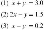
Equations (11.16) relate the two unknowns, x and y, to the observed quantities 3.0, 1.5, and 0.2. One equation is redundant since the values for x and y can be obtained from any two of the three equations. For example, if Equations (1) and (2) are solved then x would equal 1.5 and y would equal 1.5, but if Equations (2) and (3) are solved then x would equal 1.3 and y would equal 1.1, and if Equations (1) and (3) are solved then x would equal 1.6 and y would equal 1.4. Based on the inconsistency of these equations, the observations must contain errors. Therefore, new expressions, called observation equations, can be rewritten that include residuals. The resulting set of equations is

Equations (11.17) relate the unknown parameters to the observations and their errors. Equations of this form are known as residual equations. Obviously, it is possible to select values of v1, v2, and v3 that will yield the same values for x and y no matter which pair of equations are used. For example, to obtain consistencies through all of the equations, arbitrarily let v1 = 0, v2 = 0, and v3 = −0.2. In this arbitrary solution, x would equal 1.5 and y would equal 1.5, no matter which pair of equations is solved. This is a consistent solution; however, there are other values for the residuals (v's) that will produce a smaller sum of squares, and thus the most probable values for the unknowns x and y.
To find the least squares solution for x and y, the residual equations are squared and these squared expressions are added to give a function, f(x, y) that equals the ∑v2. Doing this for Equations (11.17) yields
As discussed previously, to minimize a function, its derivatives must be set equal to zero. Thus, in Equation (11.18), the partial derivatives of Equation (11.18) with respect to each unknown must be taken, and set equal to zero. This leads to the two equations:

Equations (11.19) are called normal equations. Simplifying those gives reduced normal equations of

The simultaneous solution of Equations (11.20) yields x equal to 1.514 and y equal to 1.442. Substituting these adjusted values into the residual equations [Equations (11.17)] results in the numerical values for the three residuals. Table 11.1 provides a comparison of the arbitrary solution to the least squares solution. The tabulated summations of residuals squared shows that the least squares solution yields the smaller total and thus the better solution. In fact, it is the most probable solution for the unknowns based on the observations.
TABLE 11.1 Comparison of an Arbitrary and Least Squares Solution
| Arbitrary Solution | Least Squares Solution | ||
| v1 = 0.00 | |||
| v2 = 0.00 | v2 = 0.085 | ||
| ∑v2 = 0.04 | ∑v2 = 0.025 | ||
11.7 SYSTEMATIC FORMULATION OF THE NORMAL EQUATIONS
11.7.1 Equal-Weight Case
![]() In large systems of observation equations, it would be helpful to use systematic procedures to formulate the normal equations. In developing these procedures, consider the following generalized system of linear observation equations having variables of (A, B, C,…, N).
In large systems of observation equations, it would be helpful to use systematic procedures to formulate the normal equations. In developing these procedures, consider the following generalized system of linear observation equations having variables of (A, B, C,…, N).

The squares of the residuals for Equations (11.21) are

Summing Equations (11.22), the function ![]() is obtained. This expresses the equal-weight least squares condition as
is obtained. This expresses the equal-weight least squares condition as

According to least squares theory, the minimum for Equation (11.23) is found by setting the partial derivatives of the function with respect to each unknown equal to zero. This results in the following normal equations:

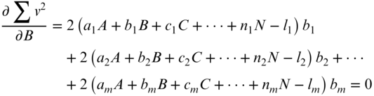

Dividing each expression by 2 and regrouping the remaining terms in Equation (11.24) results in Equation (11.25):

Generalized equations expressing normal Equations (11.25) are now written as

In Equation (11.26) the a's, b's, c's,…, n's are the coefficients for the unknowns A, B, C,…, N; the l values are the observations; and ∑ signifies the summation from i = 1 to m.
11.7.2 Weighted Case
In a manner similar to that of Section 11.7.1, it can be shown that normal equations can be systematically formed for weighted observation equations in the following manner:

In Equation (11.27), w are the weights of the observations, l; a's, b's, c's,…, n's are the coefficients for the unknowns A, B, C,…, N; l values are the observations; and ∑ signifies the summation from i = 1 to m.
Notice that the terms in Equations (11.27) are the same as those in Equations (11.26) except for the addition of the w's, which are the relative weights of the observations. In fact, Equations (11.27) can be thought of as the general set of equations for forming the normal equations, since if the weights are equal, they can all be given a value of 1. In this case, they will cancel out of Equations (11.27) to produce the special case given by Equations (11.26).
11.7.3 Advantages of the Systematic Approach
Using the systematic methods just demonstrated, the normal equations can be formed for a set of linear equations without writing the residual equations, compiling their summation equation, or taking partial derivatives with respect to the unknowns. Rather, for any set of linear equations, the normal equations for the least squares solution can be written directly.
11.8 TABULAR FORMATION OF THE NORMAL EQUATIONS
Formulation of normal equations from observation equations can be simplified further by handling Equations (11.26) and (11.27) in a table. In this way, a large quantity of numbers can be easily be manipulated. Tabular formulation of the normal equations for the example in Section 11.4.1 is illustrated below. First, Equations (11.17) are made compatible with the generalized form of Equations (11.21). These equations, the so-called observation equations, are shown in Equations (11.28).

In Equations (11.28), there are two unknowns, x and y, with different coefficients for each equation. Placing the coefficients and the observations, l's, for each expression of Equation (11.28) into a table, the normal equations are formed systematically. Table 11.2 shows the coefficients, appropriate products, and summations in accordance with Equations (11.26).
TABLE 11.2 Tabular Formation of Normal Equations
| Eqn. | a | b | L | a2 | ab | b2 | al | bl |
| (7) | 1 | 1 | 3.0 | 1 | 1 | 1 | 3.0 | 3.0 |
| (8) | 2 | −1 | 1.5 | 4 | −2 | 1 | 3.0 | −1.5 |
| (9) | 1 | −1 | 0.2 | 1 | −1 | 1 | 0.2 | −0.2 |
| ∑a2 = 6 | ∑ab = −2 | ∑b2 = 3 | ∑al = 6.2 | ∑bl = 1.3 |
After substituting the appropriate values for ∑a2, ∑ab, ∑b2, ∑al, and ∑bl from Table 11.2 into Equations (11.26), the following normal equations are

Notice that Equations (11.29) are exactly the same as those obtained in Section 11.6 using the theoretical least squares method. That is, Equations (11.29) match Equations (11.20).
11.9 USING MATRICES TO FORM THE NORMAL EQUATIONS
![]() Note that the number of normal equations in a parametric least squares adjustment is always equal to the number of unknown variables. Often, the system of normal equations becomes quite large. But even when dealing with three unknowns, their solution by hand is time-consuming. As a consequence, computers and matrix methods as described in Appendixes A through C are almost always used today. In the following subsections, we present the matrix methods used in performing a least squares adjustment.
Note that the number of normal equations in a parametric least squares adjustment is always equal to the number of unknown variables. Often, the system of normal equations becomes quite large. But even when dealing with three unknowns, their solution by hand is time-consuming. As a consequence, computers and matrix methods as described in Appendixes A through C are almost always used today. In the following subsections, we present the matrix methods used in performing a least squares adjustment.
11.9.1 Equal-Weight Case
To develop the matrix expressions for performing least squares adjustments, an analogy will be made with the systematic procedures demonstrated in Section 11.7. For this development, let a system of observation equations be represented by the matrix notation
where

Note that the above system of observation equations (11.30) is identical to Equations (11.21) except that the unknowns are x1, x2,…, xn instead of A, B,…, N, and the coefficients of the unknowns are a11, a12,…, a1n instead of a1, b1,…, n1.
Subjecting the above matrices to the manipulations given in the following expression, Equation (11.31) produces the normal equations [i.e., matrix Equation (11.31a) is exactly equivalent to Equations (11.26)]:
Equation (11.31a) can also be expressed as
where N represents the normal matrix. The correspondence between Equations (11.31) and Equations (11.26) becomes clear if the matrices are multiplied and analyzed as follows:

The individual elements of the normal matrix can be expressed in the following summation forms:
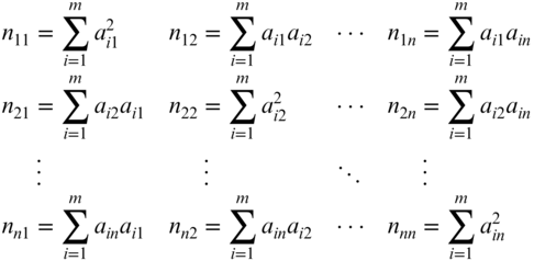
By comparing the summations above with those obtained in Equations (11.26), it should be clear that they are the same. Therefore, it is demonstrated that Equations (11.31a) and (11.31b) produce the normal equations of a least squares adjustment. By inspection, it can also be seen that the normal matrix is always symmetric (i.e., nij = nji).
By employing matrix algebra, the solution of normal equations like Equation (11.31a) is
11.9.2 Weighted Case
A system of weighted linear observation equations can be expressed in matrix notation as
Using the same methods as demonstrated in Section 11.9.1, it is possible to show that the normal equations for this weighted system are
Equation (11.34a) can also be expressed as
where N = (ATWA) is the so-called normal matrix.
By employing matrix algebra, the least squares solution of these weighted normal equations is
In Equation (11.35), W is the weight matrix as defined in Chapter 10.
11.10 LEAST SQUARES SOLUTION OF NONLINEAR SYSTEMS
![]() In Appendix C, a method is presented to solve a nonlinear system of equations using a first-order Taylor series approximation of the nonlinear equation. Following this procedure, the least squares solution for a systems of nonlinear equations can be found as follows:
In Appendix C, a method is presented to solve a nonlinear system of equations using a first-order Taylor series approximation of the nonlinear equation. Following this procedure, the least squares solution for a systems of nonlinear equations can be found as follows:
- Step 1: Write the first-order Taylor series approximation for each equation.
- Step 2: Determine initial approximations for the unknowns in the equations of Step 1.
- Step 3: Use matrix methods similar to those discussed in Section 11.9, to find the least squares solution for the equations of Step 1 (these are corrections to the initial approximations).
- Step 4: Apply the corrections to the initial approximations.
- Step 5: Repeat Steps 3 through 4 until the corrections become sufficiently small.
A system of nonlinear equations that are linearized by a Taylor series approximation can be written as
where the Jacobian matrix J contains the coefficients of the linearized observation equations. The individual matrices in Equation (11.36) are

The vector of least squares corrections in the equally weighted system of Equation (11.36) is given by
Similarly, the system of weighted equations is
and its solution is
where W is the weight matrix as defined in Chapter 10. Notice that the least squares solution of a nonlinear system of equations is similar to the linear case. In fact, the only difference is the use of the Jacobian matrix J rather than the coefficient matrix A and the use of the K matrix rather than the observation matrix, L. Many authors use the same nomenclature for both the linear and nonlinear cases. In these cases, the differences in the two systems of equations are stated implicitly.
11.11 LEAST SQUARES FIT OF POINTS TO A LINE OR CURVE
![]() Frequently in engineering work, it is desirable or necessary to fit a straight line or curve to a set of points with known coordinates. In solving this type of problem, it is first necessary to decide on the appropriate functional model for the data. The decision whether to use a straight line, parabola, or some other higher-order curve can generally be made after plotting the data and studying their form or by checking the size of the residuals after the least squares solution with the first selected line or curve.
Frequently in engineering work, it is desirable or necessary to fit a straight line or curve to a set of points with known coordinates. In solving this type of problem, it is first necessary to decide on the appropriate functional model for the data. The decision whether to use a straight line, parabola, or some other higher-order curve can generally be made after plotting the data and studying their form or by checking the size of the residuals after the least squares solution with the first selected line or curve.
11.11.1 Fitting Data to a Straight Line
Consider the data illustrated in Figure 11.2. The straight line shown in the figure can be represented by this equation:

FIGURE 11.2 Fitting points on a line.
In Equation (11.40), x and y are the coordinates of a point, m is the slope of a line, and b is the y intercept at x = 0. If the points were truly linear, and there were no observational or experimental errors, all coordinates would lie on a straight line. However, this is rarely the case, as seen in Figure 11.2, and thus, it is possible that (1) the points contain errors, (2) the functional model is a higher-order curve, or both. If a line is selected as the model for the data, the equation of the best-fitting straight line is found by adding residuals to Equations (11.40). This accounts for the errors shown in the figure. Observation equations for the four data points A, B, C, and D of Figure 11.2 are rewritten as

Equations (11.41) contain two unknowns, m and b, with four observations. Their matrix representation is
where

Equation (11.42) is solved by the least squares method using Equation (11.32). If some data were more reliable than others, relative weights could be introduced and a weighted least squares solution could be obtained using Equation (11.35).
11.11.2 Fitting Data to a Parabola
For certain data sets or in special situations, a parabola will fit the situation best. An example would be fitting a vertical curve to an existing roadbed. The general equation of a parabola is
Again, since the data rarely fit the equation exactly, residuals are introduced. For the data shown in Figure 11.3, the following observation equations can be written:


FIGURE 11.3 Fitting points on a parabolic curve.
Equations (11.44) contain three unknowns, A, B, and C, with five equations. Thus, this represents a redundant system that can be solved using least squares. In terms of the unknown coefficients, Equations (11.44) are linear and can be represented in matrix form as
Since this is a linear system, it is solved using Equation (11.32). If weights were introduced, Equation (11.35) would be used. The steps taken would be similar to those used in Section 11.11.1.
11.12 CALIBRATION OF AN EDM INSTRUMENT
Calibration of an EDM is necessary to ensure confidence in the distances it measures. In calibrating these devices, if they internally make corrections and reductions for atmospheric conditions, Earth curvature, and slope, it is first necessary to determine if these corrections are made properly. Once these corrections are applied properly, the instruments with their reflectors must be checked to determine their constant and scaling corrections. This is often accomplished using a calibration baseline. The observation equation for an electronically observed distance on a calibration baseline is
In Equation (11.46), S is a scaling factor for the EDM; C is an instrument–reflector constant; DH is the observed horizontal distance with all atmospheric and slope corrections applied; DA is the published horizontal calibrated distance for the baseline; and VDH is the residual error for each observation. This is a linear equation with two unknowns, S and C. Systems of these equations can be solved using Equation (11.31).
11.13 LEAST SQUARES ADJUSTMENT USING CONDITIONAL EQUATIONS
As stated in Section 11.5, observations can also be adjusted using conditional equations. In this section, this form of adjustment is demonstrated by using the condition that the sum of the angles in the horizon at a single station must equal 360°.
11.14 THE PREVIOUS EXAMPLE USING OBSERVATION EQUATIONS
Example 11.5 can also be done using observation equations. In this case, the three observations are related to their adjusted values and their residuals by writing observation equations:

While these equations relate the adjusted observations to their observed values, they cannot be solved in this form. What is needed is the geometric constraint 2 that states that the sum of the three angles equals 360°. This can be represented in equation form as
Rearranging Equation (s) to solve for a3 yields
Substituting Equation (t) into Equations (r) produces

This is a linear problem, with two unknowns, a1 and a2. The weighted observation equation solution is obtained by solving Equation (11.35). The appropriate matrices for this problem are

Performing the matrix manipulations, the matrices for the normal equations are

Finally, X is computed as

Using Equation (t), it can now be determined that a3 is 360° − 134°39′00.2″ − 83°17′44.1″ = 142°03′15.7″. The same results are obtained as in Section 11.13. It is important to note that no matter what method of least squares adjustment is used, if the procedures are performed properly, the same solution will always be obtained. This example involved constraint equation (t). This topic is covered in more detail in Chapter 20.
11.15 SOFTWARE
As was initially stated, the method of least squares was not used commonly due to its computational intensiveness. Today, software has eliminated this hindrance. On the companion website the spreadsheet in the file Chapter 11.xls demonstrates the least squares solution to the example problems in this chapter. It uses several of the techniques discussed in Section 8.6 to manipulate the matrices. Additionally, on the companion website is the Mathcad® worksheet C11.xmcd, which demonstrates the programming of all of the examples in this chapter. These examples should be studied by the reader. Similar programming can be used to solve the problems at the end of this chapter. For those who wish to create a more robust program, a higher-level programming language can be used.
Both spreadsheet and Mathcad® software are available for the reader in many of the remaining chapters. The spreadsheet software files are named as Chapter##.xls where ## represents the chapter number. The Mathcad® worksheets are similarly named after their representative chapter. These files demonstrate some of the programming techniques that are used to solve the example problems in this book. Readers are encouraged to investigate these files while studying the subject material in this book.
PROBLEMS
Note: Partial answers to problems marked with an asterisk can be found in Appendix H.
- *11.1 Calculate the most probable values for A and B in the equations below by the method of least squares. Consider the observations to be of equal weight. (Use the tabular method to form normal equations.)
- (a) 3A + 2B = 7.8 + v1
- (b) 2A − 3B = 2.5 + v2
- (c) 6A − 7B = 8.5 + v3
- 11.2 If observations a, b, and c in Problem 11.1 have weights of 2, 4, and 5, respectively, solve the equations for the most probable values of A and B using weighted least squares. (Use the tabular method to form normal equations.)
- 11.3 Repeat Problem 11.1 using matrices.
- 11.4 Repeat Problem 11.2 using matrices.
- 11.5 Calculate the most probable values of X and Y for the following system of equations using
- (a) Tabular method.
- (b) Matrix method.

- *11.6 What are the residuals for the system of equations in Problem 11.5?
- *11.7 Solve the following nonlinear equations using the least squares method. Use initial approximations of x0 = 2.1 and y0 = 0.45.

- 11.8 What are the residuals for the system of equations in Problem 11.7?
- 11.9 Repeat Problem 11.7 for the following system of nonlinear equations using initial approximations of x0 = 2.8 and y0 = 5.6.

- 11.10 If observations 1, 2, and 3 in Problem 11.9 have weights of 3, 2, and 1, respectively, solve the equations for:
- (a) the most probable values of x and y.
- (b) the residuals.
- 11.11 The following coordinates of points on a line were computed for a block. What are the slope and y-intercept of the line? What is the azimuth of the line?
Point X (ft) Y (ft) 1 1254.72 3373.22 2 1362.50 3559.95 3 1578.94 3934.80 4 1843.68 4393.35 - *11.12 Using the conditional equations, what are the most probable values for the three angles observed to close the horizon at station Red. The observed values and their standard deviations are
Angle Value S (″) 1 114°23′05″ ±6.5 2 138°17′59″ ±3.5 3 107°19′03″ ±4.9 - 11.13 Do Problem 11.12 using the observation equation method.
- 11.14 Using the conditional equation method, what are the most probable values for the three interior of a triangle that were measured as:
Angle 15 S (″) 1 65°23′56″ ±7.6 2 83°15′43″ ±4.3 3 31°21′12″ ±8.4 - 11.15 Do Problem 11.14 using the observation equation method.
- 11.16 Eight blocks of the Main Street are to be reconstructed. The existing street consists of jogging, short segments as tabulated in the traverse survey data below. Assuming coordinates of X = 1000.0 and Y = 1000.0 at station A, and that the azimuth of AB is 90°, define a new straight alignment for a reconstructed street passing through this area that best conforms to the present alignment. Give the Y intercept and the azimuth of the new alignment.
Course Length (ft) Station Angle to Right AB 635.74 B 180°01′26″ BC 364.82 C 179°59′52″ CD 302.15 D 179°48′34″ DE 220.08 E 180°01′28″ EF 617.36 F 179°59′05″ FG 429.04 G 180°01′37″ GH 387.33 H 179°59′56″ HI 234.28 - 11.17 Use the ADJUST software to do Problem 11.16.
- 11.18 The property corners on a single block with an alley are shown as a straight line with a Due East bearing on a recorded plat. During a recent survey, all the lot corners were found, and measurements from the Station A to each were obtained. The surveyor wants to determine the possibility of disturbance of the corners by checking their fit to a straight line. A sketch of the situation is shown in Figure 11.4, and the results of the survey are given below. Assuming Station A has coordinates of X = 5000.00 and Y = 5000.00, and that the coordinates of the backsight station are X = 5000.10 and Y = 5200.00, determine the best fitting line for the corners. Give the Y intercept and the azimuth of the best-fit line.
Course Distance (ft) Angle at A AB 100.02 90°00′16″ AC 200.12 90°00′08″ AD 300.08 89°59′48″ AE 399.96 90°01′02″ AF 419.94 89°59′48″ AG 519.99 90°00′20″ AH 620.04 89°59′36″ AI 720.08 90°00′06″ 
- 11.19 Use the ADJUST software to do Problem 11.18.
- 11.20 Using a procedure similar to that in Section 11.7.1, derive Equations (11.27).
- 11.21 Using a procedure similar to that used in Section 11.9.1, show that the matrix operations in Equation (11.34) result in the normal equations for a linear set of weighted observation equations.
- 11.22 Discuss the importance of selecting the stochastic model when adjusting data.
- 11.23 The values for three angles in a triangle, observed using a total station, are
Angle Number of Repetitions Value A 2 14°25′20″ B 4 58°16′00″ C 4 107°19′10″ - The observed lengths of the course are

- The following estimated errors are assumed for each measurement:

What are the most probable values for the angles? Use the condition equation method.
- The observed lengths of the course are
- 11.24 Do Problem 11.23 using observation equations and a constraint as presented in Section 11.13.
- 11.25 The following data were collected on a calibration baseline. Atmospheric refraction and Earth curvature corrections were made to the measured distances, which are in units of meters. Determine the instrument/reflector constant and any scaling factor.
Distance DA DH Distance DA DH 0 – 150 149.9104 149.9447 150 – 0 149.9104 149.9435 0 – 430 430.0010 430.0334 430 – 0 430.0010 430.0340 0 – 1400 1399.9313 1399.9777 1400 – 0 1399.9313 1399.9519 150 – 430 280.0906 208.1238 430 – 150 280.0906 280.1230 150 – 1400 1250.0209 1250.0795 1400 – 150 1250.0209 1250.0664 430 – 1400 969.9303 969.9546 1400 – 430 969.9303 969.9630 - 11.26 A survey of the centerline of a horizontal curve is done to determine the as-built curve specifications. The coordinates for the points along the curve are:
Point X (ft) Y (ft) 1 9,821.68 9,775.84 2 9,876.40 9,842.74 3 9,975.42 9,955.42 4 10,079.50 10,063.40 5 10,151.60 10,132.68 - (a) Using Equation (C.10), compute the most probable values for the radius and center of the circle.
- (b) If two points located on the tangents have coordinates of (9761.90, 9700.66) and (10,277.88, 10,245.84), what are the coordinates of the PC and PT of the curve?